
Featured Viscous Pipe Flow Resources
[no_toc]

Orifice Meter Working Principles and Applications
Types of Volumetric Flow Meters: Measuring Fluids with Precision
Venturi Flow Meters: A Comprehensive Introduction

Colebrook-White Equation
Moody Chart for Estimating Friction Factors

Loss Coefficients: A Practical Guide for Engineers

Hazen-Williams Equation Explained
Moody Chart Calculator
Hagen-Poiseuille Equation: Essential Guide for Fluid Dynamics

Equivalent Lengths of Pipe Fittings
Viscous pipe flow is a crucial aspect of fluid dynamics in pipe systems, which involves the transport of liquids or gases through enclosed conduits. The viscosity of the fluid, along with factors like pipe diameter, roughness, and flow velocity, plays a vital role in classifying the flow as laminar or turbulent.
A key parameter for evaluating pipe flow is the Reynolds number (Re), defined as the ratio of inertial forces to viscous forces. Mathematically, it can be expressed as:
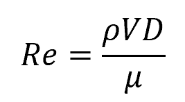
Where:

Elevate Your Engineering With Excel
Advance in Excel with engineering-focused training that equips you with the skills to streamline projects and accelerate your career.
- ρ is the fluid density,
- V is the average velocity,
- D is the pipe diameter, and
- μ is the dynamic viscosity of the fluid.
In general, a Reynolds number less than 2300 indicates laminar flow, while a value greater than 4000 signifies turbulent flow.
Principles of Laminar and Turbulent Flow
Viscous pipe flow can be classified into three primary flow regimes: laminar flow, transitional flow, and turbulent flow. Each of these regimes exhibits different fluid behaviors that can influence the performance and design of engineering systems.
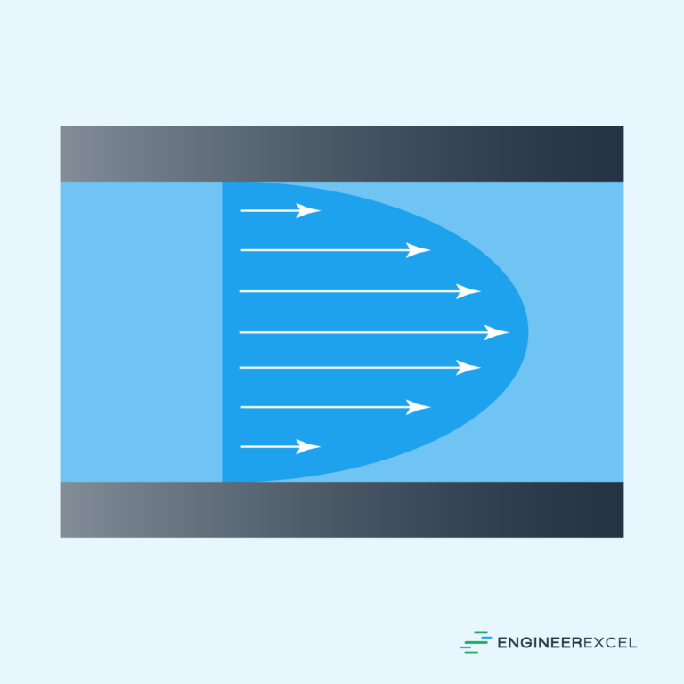
Laminar flow is characterized by smooth, orderly, and parallel fluid motion, typically occurring at low Reynolds numbers (Re < 2300) source. In this regime, viscous forces dominate the flow, leading to a stable and predictable fluid velocity profile. One of the key properties of laminar flow is the parabolic velocity profile, with the maximum velocity at the center of the pipe and zero velocity at the pipe’s walls.
Transitional flow occurs over a range of Reynolds numbers (2300 < Re < 4000), where both laminar and turbulent behaviors can be observed. In this region, disturbances or small perturbations in the flow can cause the regime to switch between laminar and turbulent flow.
Turbulent flow is characterized by chaotic and irregular fluid motion, typically at higher Reynolds numbers (Re > 4000). In this regime, inertial forces play a more dominant role, resulting in the formation of eddies and vortices throughout the flow source. The velocity profile in turbulent flow becomes flatter and less predictable compared to laminar flow.
For both laminar and turbulent flow, it is important to understand the concept of fully developed flow.
Flow Entrance & Development
The entrance length is the distance from the beginning of the pipe, where the fluid enters the pipe, to the point where the flow becomes fully developed. In a fully developed flow, the velocity profile does not change along the pipe’s length. It is crucial to note that the entrance length depends on the flow’s Reynolds number. In general, the entrance length is shorter for laminar flows compared to turbulent flows.
During the development of the flow, two regions can be identified within the pipe. The first region is the entrance region, also known as the hydrodynamic entry length, where the flow undergoes changes in velocity profile as it adjusts to the pipe’s geometry. In this region, the boundary layer gradually grows and approaches the pipe’s centerline. Consequently, the pressure drop within the entrance region is not constant.
The second region is the fully developed region, where the velocity profile remains constant along the pipe’s length and the boundary layers have merged. As a result, the pressure drop in this region is constant. In practical applications, engineers often focus on the fully developed region, as the flow characteristics, such as pressure drop and friction factor, become predictable and consistent.
Major and Minor Losses in Flow
Pressure losses occur due to the friction between the fluid and the walls of the pipe. These losses are classified into two categories: major losses and minor losses.
Major losses are associated with the resistance caused by the pipe itself, and they depend on factors like pipe diameter, length, internal surface roughness, and fluid viscosity. These losses can be quantified using the Darcy-Weisbach equation:
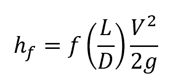
where hf is the head loss, f is the friction factor, L is the pipe length, D is the pipe diameter, V is the average flow velocity, and g is the acceleration due to gravity. The friction factor can be determined experimentally via the Moody chart or calculated using the Colebrook-White equation for turbulent flow and the Hagen-Poiseuille equation for laminar flow.
Minor losses, on the other hand, result from the flow resistance induced by pipe fittings, valves, bends, and other disturbances in the flow path. These losses are typically reported in terms of coefficients, which are multiplied by the dynamic pressure, to estimate the pressure loss. The head loss due to these minor losses can be expressed as:

where hm is the minor head loss and K is the loss coefficient. For various types of fittings and flow configurations, the values of the loss coefficients can be found in handbooks and engineering resources.
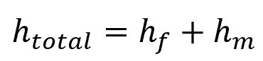
In piping systems containing both major and minor losses, the total head loss is the sum of the individual losses:
In some cases, minor losses can be significant, even dominating the pressure drop, especially in complex systems with numerous fittings and devices.
Equivalent Length

Losses due to pipe components can be quantified using the concept of equivalent length. This is done by determining how much straight pipe would produce the same pressure loss as the fitting, valve, or component in question. The equivalent length of each component can then be added to the total length of the pipe, resulting in a modified pipeline length for calculating the head loss. The head loss calculation can then be performed using well-established formulas like the Darcy-Weisbach equation or the Hazen-Williams formula.
The equivalent length of a specific pipe component is commonly expressed as a multiple of the pipe’s diameter (for example, Le/D). Engineers can find these values in published resources and literature which provide tables of equivalent lengths for various types of fittings and valves. A sample of such data is presented below:
| Pipe Component | Equivalent Length (Le/D) |
|---|---|
| 90° Elbow | 30 |
| 45° Elbow | 16 |
| Tee | 60 |
| Gate Valve | 8 |
| Globe Valve | 340 |
These equivalent length values are often dependent on factors such as the Reynolds Number, which characterizes the flow regime (laminar or turbulent) and the relative roughness of the pipe’s inner surface. This further influences the values of the friction factor, which should be carefully chosen based on the specific flow conditions to ensure accurate predictions.
Role of Pipe Roughness
Pipe roughness plays a major role in determining the flow characteristics and head losses in viscous pipe flow. It is a measure of the irregularities present on the inner surface of the pipe. These irregularities affect the fluid flow and cause the velocity distribution to deviate from the ideal laminar or turbulent patterns. The relative roughness of a pipe, defined as the ratio of the pipe’s surface roughness to its diameter, is a key parameter in evaluating the impact of pipe roughness on the flow.
Different types of pipes have varying degrees of roughness, depending on the material and manufacturing process used. This roughness can have a significant effect on the head loss in pipe flow systems. Head loss refers to the decrease in fluid pressure due to friction between the fluid and the pipe walls. As the roughness of the pipe increases, the frictional resistance to fluid flow also increases, resulting in higher head loss.
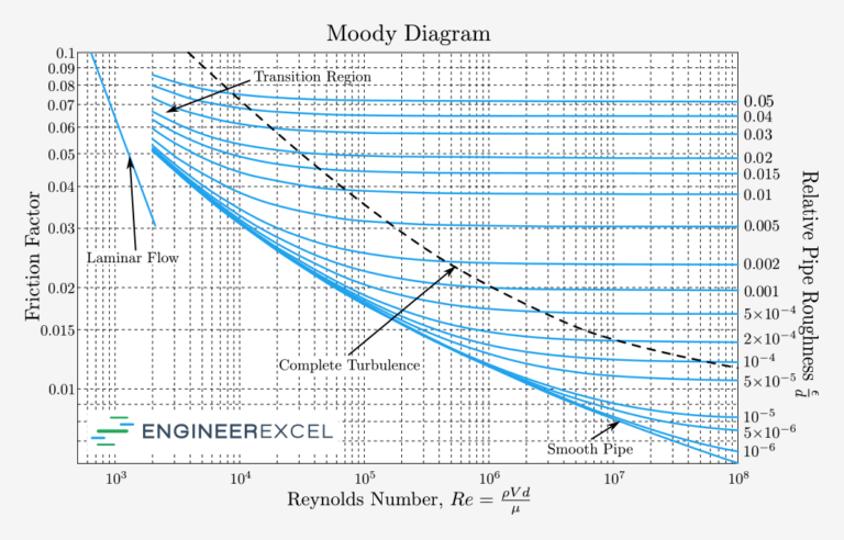
The understanding and quantification of pipe roughness are essential for accurate prediction of fluid flow behavior and head loss in engineering applications. Engineers use the Moody diagram and friction factor calculations to account for the effect of pipe roughness in flow analysis and design. The Moody diagram is a graphical representation of the relationship between the Reynolds number, relative roughness, and friction factor, which aids in determining the head loss in pipe flow systems.
Furthermore, the impact of pipe roughness on flow transitions is noteworthy. As the roughness increases, the transition from laminar to turbulent flow occurs at lower Reynolds numbers. Laminar flow is characterized by smooth, orderly fluid motion, while turbulent flow involves more chaotic, disordered motion. Turbulent flow is associated with higher energy losses due to the increased friction and mixing between fluid layers, making the consideration of pipe roughness essential for achieving efficient system performance.
Insights into the Colebrook-White Equation
The Colebrook-White equation is an implicit and complex formula in fluid mechanics that predicts the friction factor (f) in turbulent pipe flow, depending on the Reynolds number (Re) and the pipe’s relative roughness (ε/D). It is widely used by engineers and scientists in numerous applications, from hydraulics to chemical engineering.
The equation takes the form:
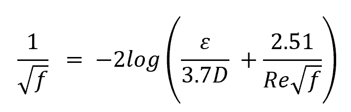
Here, f is the friction factor, Re is the Reynolds number, and ε/D represents the relative roughness of the pipe.
There are multiple methods to solve the Colebrook-White equation, given its complex and non-linear nature. One popular solution method is using iterative techniques such as the Newton-Raphson or Bisection method. Alternatively, engineers utilize the Moody Diagram as a graphical representation of the Colebrook-White equation to estimate the friction factor quickly.
Several explicit approximations available simplify the Colebrook-White equation, such as the Swamee-Jain equation or Blasius equation. While these simplified equations are more manageable, they may lack accuracy compared to the original Colebrook-White equation.
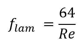
For laminar flow the equation can be replaced with Hagen-Poiseuille equation:
Understanding the Moody Chart
The Moody Chart provides a graphical representation of the friction factor as a function of the Reynolds number and relative roughness of the pipe. This allows engineers to easily and quickly determine the friction factor.
The chart is divided into three distinct regions: laminar flow, transition flow, and turbulent flow. Each of these regions is characterized by different relationships between the Reynolds number, relative roughness, and friction factor.
- Laminar Flow (Re ≤ 2,300): In this region, the friction factor can be calculated using the expression f = 16 / Re.
- Transition Flow (2,300 < Re ≤ 4,000): It is difficult to predict the friction factor for transitional flow precisely, but the Moody Chart provides approximate values for this range.
- Turbulent Flow (Re > 4,000): In this region, the friction factor depends on both the Reynolds number and the relative roughness (ε/D), which is the ratio of the pipe’s roughness height (ε) to its diameter (D). The Moody Chart presents an array of curves representing various values of relative roughness.
To use the Moody Chart, follow these steps:
- Determine the Reynolds number (Re) using the formula: Re = ρVD/μ, where ρ is the fluid density, V is the average flow velocity, D is the pipe diameter, and μ is the dynamic viscosity.
- Calculate the relative roughness (ε/D) using the known values of ε (typically provided by the pipe manufacturer) and the pipe diameter (D).
- Locate the Reynolds number on the x-axis and the relative roughness on the right side of the chart.
- Draw a vertical line from the Reynolds number and a horizontal line from the relative roughness. The intersection of these lines will fall on a curve that represents the friction factor.
- Read the friction factor value from the left side of the chart.
It is crucial to mention that the Moody Chart should be used with caution in the transition flow region, as the values in this range might not be as accurate. However, for most practical applications in the laminar and turbulent flow regions, the Moody Chart remains a valuable and reliable resource for estimating the friction factor and predicting pipe flow behavior.
Hazen Williams Equation
The Hazen Williams Equation is an empirical formula often used in civil engineering for the estimation of the flow rate in pipes. This approximation provides an efficient way to determine head loss and pressure drop in fluid flow situations, particularly for water distribution systems under steady state conditions. The equation takes into account the pipe material, diameter, and flow velocity, enabling engineers to design and optimize water supply systems.
The Hazen Williams Equation in SI units is given by the following formula:
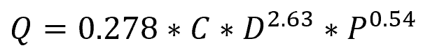
where Q represents the flow rate (m^3/s), C is the Hazen Williams coefficient, which accounts for the pipe roughness, D is the pipe diameter (m), and P is the head loss per unit length of the pipe (Pa/m). The Hazen Williams coefficient (C) depends on the type of pipe material, with higher values indicating smoother surfaces, leading to lower head loss and frictional effects. For instance, new plastic pipes might have a C value of 150, while older cast iron pipes may have a value of 100.
Some limitations of the Hazen Williams Equation should be noted. First, it is only valid for water at normal temperatures, and hence, does not account for variations due to fluid properties like viscosity and density. Second, the empirical nature of the equation means it might not be as accurate under extreme conditions, or for pipes made of unconventional materials. In such cases, engineers may prefer to use more robust methods like the Darcy Weisbach equation.
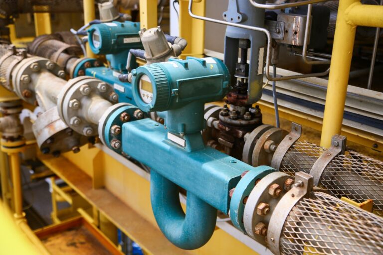
Flow Measurement Devices
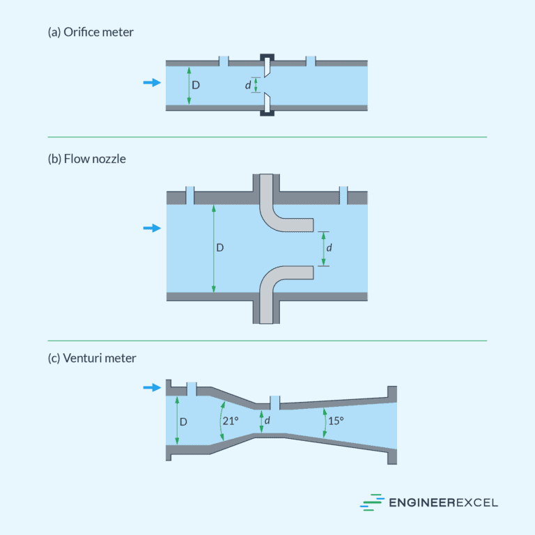
Orifice Meters
Orifice meters are used for measuring fluid flow rates in pipes. They consist of a thin plate with an opening called an orifice, which is placed perpendicular to the flow direction. When the fluid passes through the orifice, its pressure decreases due to the constriction, causing a pressure difference that can be correlated with flow velocity . This can be determined mathematically using the Bernoulli equation and continuity principle. The primary advantage of orifice meters is their relatively low cost and wide applicability to different fluids and pipe diameters.
Volumetric Flow Meters
Volumetric flow meters measure the volume of fluid that passes through a specific point in the pipe within a given time. Common types of volumetric flow meters include Positive Displacement Flow Meters and Turbine Flow Meters. Positive Displacement flow meters quantify fluid flow by dividing the fluid into fixed volumetric compartments and counting the compartments as they pass. Turbine flow meters measure fluid flow using a spinning rotor driven by the fluid velocity. The rotational speed of the rotor can be correlated with the flow rate. These flow meters are best suited for applications requiring high accuracy and continuous flow monitoring.
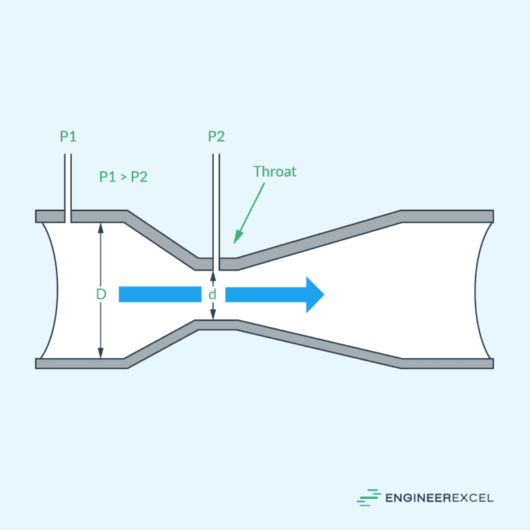
Venturi Flow Meters
A Venturi flow meter is a measurement device that uses the principle of pressure difference to determine the fluid velocity in a pipe. The Venturi meter consists of a converging section that accelerates the fluid flow, a throat section with the smallest cross-sectional area, and a diverging section. As the fluid flows through the constriction, its pressure decreases, and the pressure difference between the upstream and downstream sections is used to calculate the flow rate. Venturi flow meters have the advantage of lower permanent pressure loss compared to orifice meters and are suitable for measuring fluid flows with high velocities and low viscosities.
Nozzle Meters
Nozzle meters function similarly to Venturi meters but use a nozzle-shaped constriction instead of a Venturi tube. The nozzle meters are designed to minimize potential flow separation, loss of energy, and provide stable, accurate measurements. They can be used for high-velocity fluid flow and are particularly suitable for gas flow measurement due to the minimized pressure loss. Additionally, nozzle meters have a lower susceptibility to wear and blockage, making them ideal for fluids containing suspended particles.