Fluid flow in pipes encounters two types of losses: major losses and minor losses. Major losses arise from frictional resistance along the pipe length caused by fluid viscosity and wall roughness, while minor losses result from components, fittings, and geometric changes along the flow path.

This article specifically focuses on the loss coefficients related to minor losses, providing engineers with a practical guide to comprehend and quantify them effectively.
Loss Coefficient Explained
Minor losses, also known as local losses, refer to pressure losses that occur in a pipe due to various factors other than frictional losses along its length. These losses are associated with changes in flow direction, shape, or size of the pipe, as well as the presence of fittings, valves, and other flow control devices, along with pipe entrances and exits.
Despite being called minor losses, in certain cases, they can be more significant than major losses. For example, a series of fittings and partially closed valves can result in a greater pressure drop than the frictional resistance associated with major loss along the pipe.

Elevate Your Engineering With Excel
Advance in Excel with engineering-focused training that equips you with the skills to streamline projects and accelerate your career.
It is important to note that a single pipe can have multiple minor losses, all contributing to the overall pressure drop. These losses are quantified using dimensionless values known as loss coefficients, usually represented as “K.” Each type of valve, fitting, or component has its own specific loss coefficient.
Since the resulting flow mechanisms caused by these components along the pipeline are complex and the properties of valves and fittings can vary between manufacturers, the theory behind them is not well understood. As a result, loss coefficients are commonly determined experimentally through testing and correlated with pipe flow parameters, or obtained from established engineering references.
It is worth mentioning that the data, particularly for valves and fittings, depend on the specific manufacturer’s design. Therefore, most published values of loss coefficients are only considered as average design estimates.
While minor losses are expected to be influenced by flow properties, the literature often does not correlate the loss coefficient with the Reynolds number or roughness ratio. Instead, it is generally related simply to the size of the pipe. In fact, almost all data are reported for turbulent flow conditions only.
Minor Loss Coefficient Calculation
Using the measured pressure drop, the loss coefficient of a component can be calculated using the following formula:
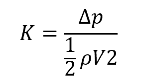
Where:
- K = loss coefficient of the component [unitless]
- Δp = pressure drop due to the component [Pa]
- ρ = fluid density [kg/m3]
- V = fluid velocity [m/s]
A pipe system typically has multiple valves, fittings, and other components that collectively contribute to minor losses. By determining the loss coefficients of each component, their individual contributions to the minor losses can be calculated. These contributions can then be combined with the major loss to determine the total system head loss.
Since both the major loss and minor loss are influenced by the velocity head, they can be summed up to obtain a single total system loss. This can be achieved using the following equation:
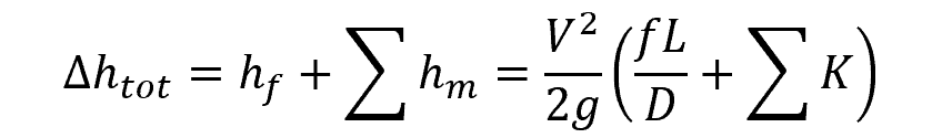
Where:
- Δhtot = total system head loss [m]
- hf = major loss due to friction [m]
- ∑hm = summation of minor losses [m]
- g = gravitational constant [9.81 m/s2]
- f = Darcy friction factor [unitless]
- L = length of the pipe [m]
- D = hydraulic diameter of the pipe [m]
Please note that the formula assumes a consistent diameter for the entire pipe system. If certain sections of the pipe system have varying diameters, the calculation must be performed on a per-section basis.
Loss Coefficient Of Valves And Fittings
A valve is a mechanical device that controls fluid flow by opening, closing, or partially obstructing the path of the flow. There are various valve geometries used in commercial applications. The five most common designs are the gate valve, globe valve, angle valve, swing-check valve, and disk valve.
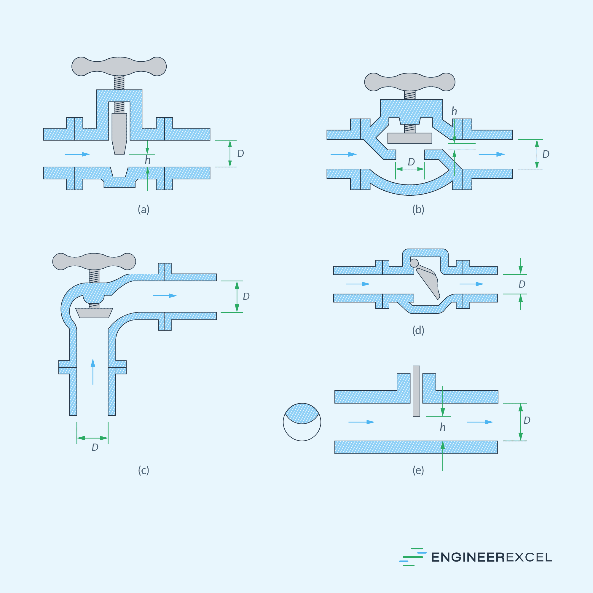
A gate valve controls flow by raising or lowering a sliding gate perpendicular to the fluid flow direction; a globe valve utilizes a movable disk or plug connected to a stem; an angle valve is similar to a globe valve, but with a 90° turn; a swing-check valve permits one-way flow through the use of a hinged disc; and a disk valve controls flow by rotating a flat or curved disk.
Among these designs, the globe valve, with its convoluted flow path, experiences the highest minor loss when fully open.
The table below shows the loss coefficients of fully open valves, elbows, and tees at different pipe sizes and configurations. In general, fittings connected by flanges have a different set of loss coefficients compared to fittings connected by internal screws.
It can be observed from the table above that the loss coefficient generally decreases with increasing pipe size. This trend is in line with the higher Reynolds number and reduced roughness ratio.
Note that the table above only includes fully open valves. For partially open valves, the loss coefficient value varies linearly, as shown on its graph versus the fractional opening below.
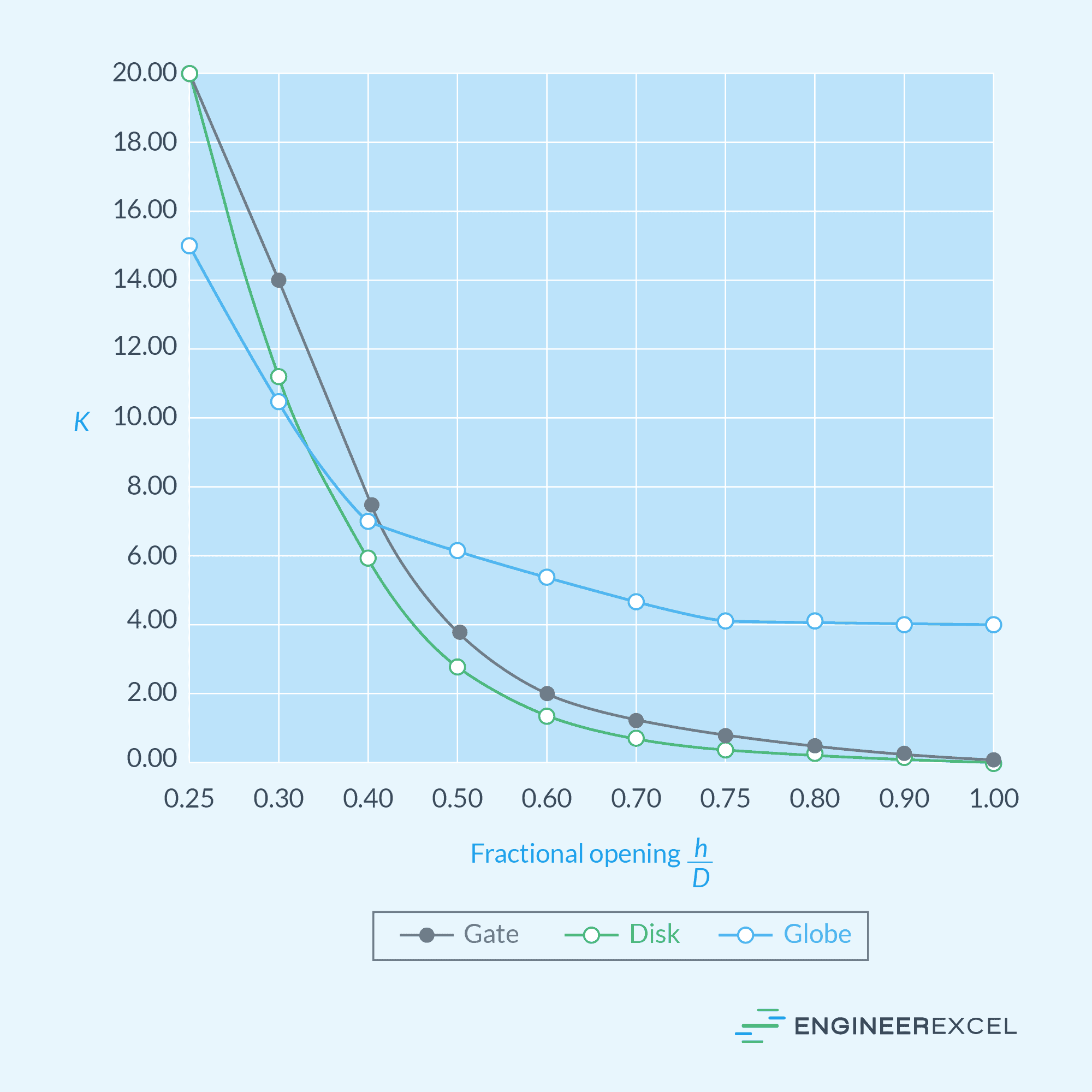
It is important to note that the loss coefficient values indicated here are only averaged among various manufacturers, which can result in an uncertainty of up to ±50 percent.
It is difficult to create an accurate list of loss coefficients as their values may differ between manufacturers and vary with advancements in fitting fabrication technology. Modern forged and molded fittings often exhibit lower loss factors. Therefore, it is advisable to rely on more updated and accurate data provided by the manufacturer.
Loss Coefficients Of Bends And Branches
Bends are curved sections in a pipe that allow for a change in direction of the fluid flow. They are typically manufactured in 45⁰ or 90⁰ curvature, although custom angles can also be created.
On the other hand, branches are tee-shaped connections where the main pipeline splits into two or more smaller pipelines. They enable the distribution of fluid to different directions or locations.
The table below shows the typical values of loss coefficients for some of the most common configurations of bends and branches.

Loss Coefficients Of Pipe Entrances And Exits
Pipe entrances and exits refer to the points where pipes begin or end within a system. The table below shows the typical values of loss coefficients for some of the most common configurations of pipe entrances and exits.

Notice that the loss coefficient for pipe exit is simply equal to the kinetic energy correction factor, α. The kinetic energy correction factor is equal to 2 for fully developed laminar flow, and 1 for fully developed turbulent flow.
Loss Coefficients Of Sudden Expansion And Contraction
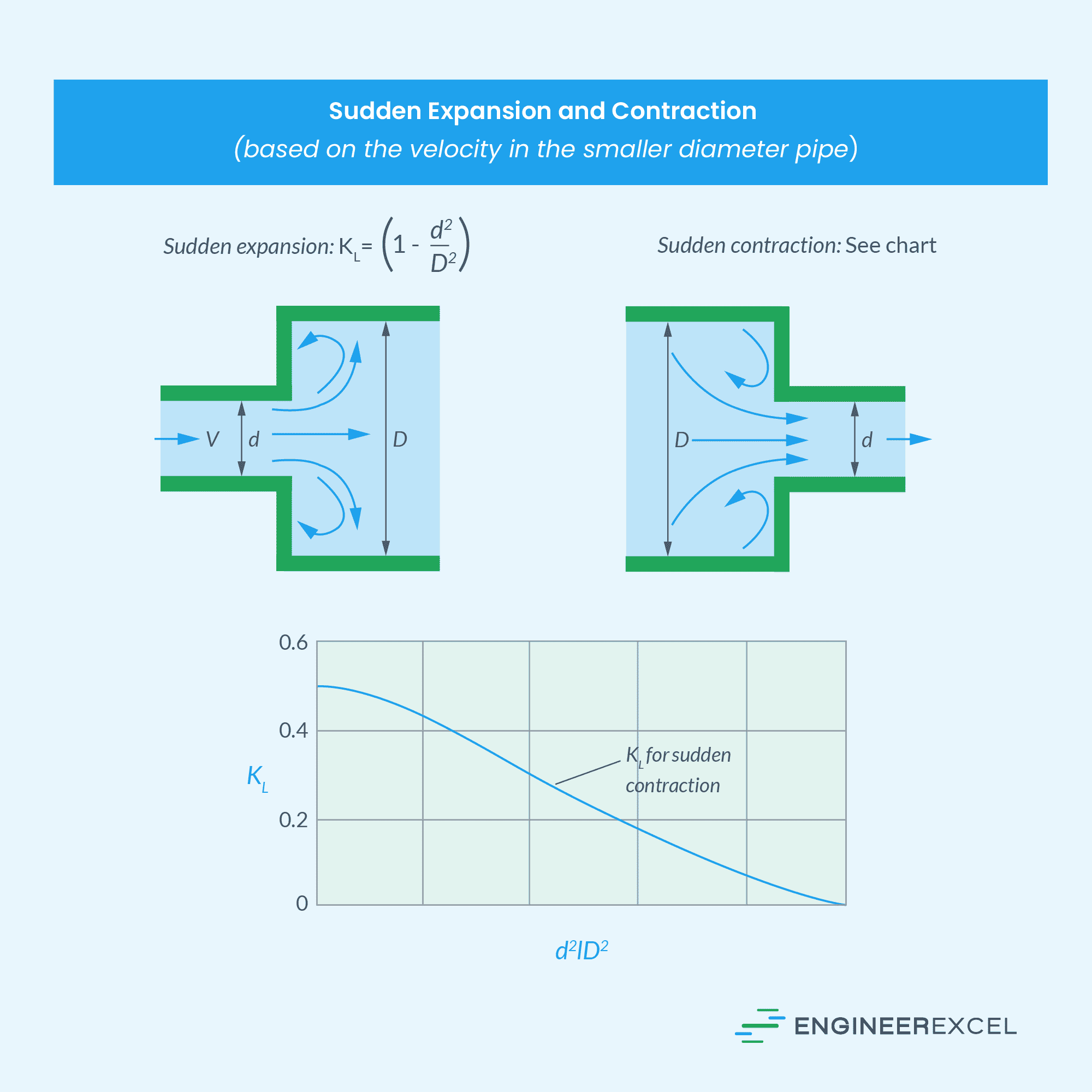
In a piping system, sudden expansion or contraction refers to a significant change in the cross-sectional area of the pipe, resulting in an abrupt change in the flow area.
Sudden expansion occurs when the pipe diameter suddenly increases, leading to a decrease in fluid velocity. On the other hand, sudden contraction occurs when the pipe diameter suddenly decreases, causing an increase in fluid velocity.
The value of the loss coefficient, in this case, is dependent on the square of the ratio of the smaller diameter and the larger diameter. For sudden expansion, the loss coefficient can be calculated using the following formula:
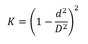
Where:
- d = diameter of the smaller cross-section [mm or in]
- D = diameter of the larger cross-section [mm or in]
For sudden contraction, the flow separation along the downstream is more complex and the loss coefficients are purely obtained from experiments. The graph of the loss coefficient against the square of the diameter ratio for sudden contraction is shown in the figure below.
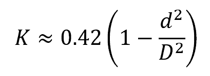
For d/D values up to 0.76, the graph above can be approximated using the following empirical formula:
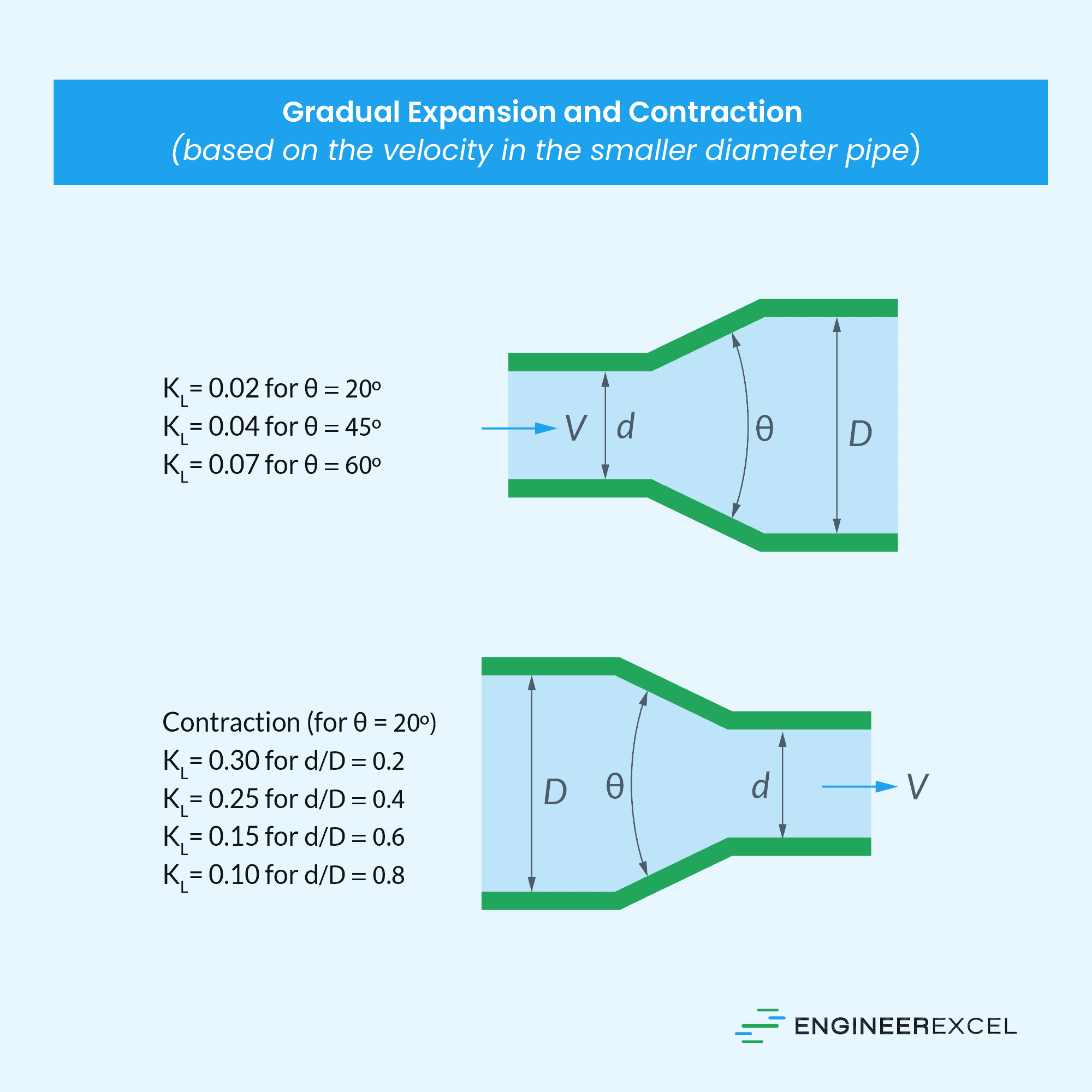
Loss Coefficients Of Gradual Expansion And Contraction
Gradual expansion and contraction in pipes refer to the gradual changes in the cross-sectional area of a pipe along its length. These changes are designed to minimize fluid flow disturbances and pressure losses compared to sudden pipe expansion or contraction.
A gradual expansion occurs when a pipe’s diameter increases gradually over a certain length. Conversely, a gradual contraction refers to a reduction in pipe diameter over a certain length.
The table below shows the typical values of loss coefficients for some of the most common configurations of gradual expansion and contraction, based on the velocity in the smaller-diameter pipe.