
Velocity and pressure are two crucial parameters that are used to characterize fluid flow in pipes. Hence, in order to design and optimize piping systems, it is important to understand the relationship between these two parameters.

This article delves into the relationship between fluid velocity and pressure, and explores the underlying principles that relate them across different flow scenarios.
Relationship Between Velocity And Pressure In Pipe Flow
The simplest and most common principle that relates pressure and fluid velocity in pipe flow is the Bernoulli’s principle— named after Daniel Bernoulli, who derived it in the 18th century. It states that as the velocity of a fluid increases, the static pressure it exerts decreases, and vice versa, assuming that the fluid’s potential energy is constant.
This principle is derived from the principle of conservation of energy and is mathematically expressed by the Bernoulli equation. The Bernoulli equation states that the total energy per unit volume, which is the sum of kinetic energy, potential energy, and internal energy, of a fluid along a streamline is constant. This is shown in the following equation:

Elevate Your Engineering With Excel
Advance in Excel with engineering-focused training that equips you with the skills to streamline projects and accelerate your career.
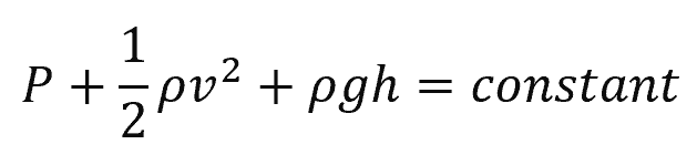
Where:
- P = pressure of the fluid at a particular point along the streamline [Pa]
- ρ = density of the fluid [kg/m3]
- v = velocity of the fluid at that point [m/s]
- g = acceleration due to gravity [9.81 m/s2]
- h = elevation of the fluid above a reference point [m]
The terms in the equation above represent various forms of energy related to fluid flow. The first term corresponds to the static pressure exerted by the fluid, the second term corresponds to the fluid’s kinetic energy due to its velocity, and the third term corresponds to the fluid’s potential energy due to its elevation.
However, the Bernoulli equation is only applicable to special situations where the flow is steady, incompressible, and frictionless. In real-world scenarios, fluid flows often involve factors such as viscosity, fluctuations, compressibility, and friction, which violate the assumptions of this equation. In these cases, the Bernoulli equation should be used with caution and its limitations must be considered.
Velocity And Pressure Relationship In Viscous Flow
In most practical applications, piping systems typically handle viscous fluids. For flows with non-negligible viscosity, the energy balance across two points should account for pressure losses due to friction, as shown in the following equation, expressed in terms of heads:
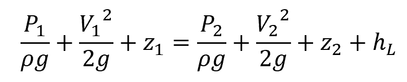
Where:
- P1, P2 = fluid pressures at points 1 and 2 [Pa]
- V1, V2 = fluid velocities at points 1 and 2 [m/s]
- z1, z2 = elevation at points 1 and 2 [m]
- hL = head loss [m]
In general, the pressure loss in fully developed internal flow is directly proportional to the square of the average fluid velocity. This relationship is depicted by the Darcy-Weisbach equation shown below:
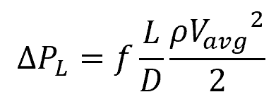
Where:
- ΔPL = pressure loss due to friction [Pa]
- f = Darcy-Weisbach friction factor [unitless]
- L = length of pipe [m]
- D = hydraulic diameter of the pipe [m]
- Vavg = average fluid velocity [m/s]
The Darcy-Weisbach friction factor is a dimensionless parameter that is a function of the Reynolds number and/or the roughness of the pipe surface, depending on the flow regime. In practical applications, it can be obtained using the Moody chart or through empirical calculations.
Velocity And Pressure Relationship In Piping Systems
The Darcy-Weisbach equation shown above applies to all types of fully developed internal flows, including laminar or turbulent flows, circular or noncircular pipes, smooth or rough surfaces, and horizontal or inclined pipes.
However, its validity is limited to straight pipes. It does not account for pressure losses resulting from valves, fittings, and other geometrical changes commonly encountered in a typical piping system. These pressure losses are referred to as minor losses.
Similar to friction-induced pressure loss, minor losses are likewise proportional to the square of the average fluid velocity, as shown in the following formula:
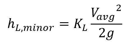
Where:
- hL, minor = minor loss due to valves, fittings, or other components [m]
- KL = loss coefficient [unitless]
The loss coefficient is a dimensionless parameter that quantifies the pressure drop resulting from components or geometric changes along a pipeline. These include valves, fittings, bends, branches, pipe inlet, pipe outlet, and changes in pipe diameter. The value of the loss coefficient depends on both the geometry and the material of the component, and it is typically determined experimentally or from empirical data.
Taking into account the minor losses and adding them with the friction-induced pressure losses, the formula for the total head loss becomes:
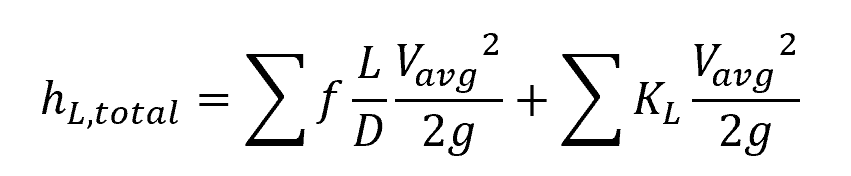
Where:
- hL,total = total head loss [m]
Velocity And Pressure Relationship In Laminar Flow
For laminar flows in a horizontal pipe, the Darcy-Weisbach formula can be simplified into an equation that relates the average velocity and the change in pressure across two points, shown below:
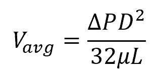
Where:
- ΔP = change in pressure between two points along a pipe [Pa]
- μ = viscosity of the fluid [Pa-s]
For laminar flows in an inclined pipe, the above equation can be modified to account for the effect of fluid weight due to the pipe’s inclination, as shown in the following equation:
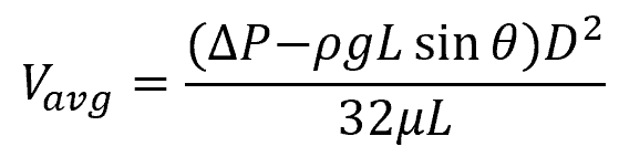
Where:
- θ = angle of inclination with respect to the horizontal [rad or deg]
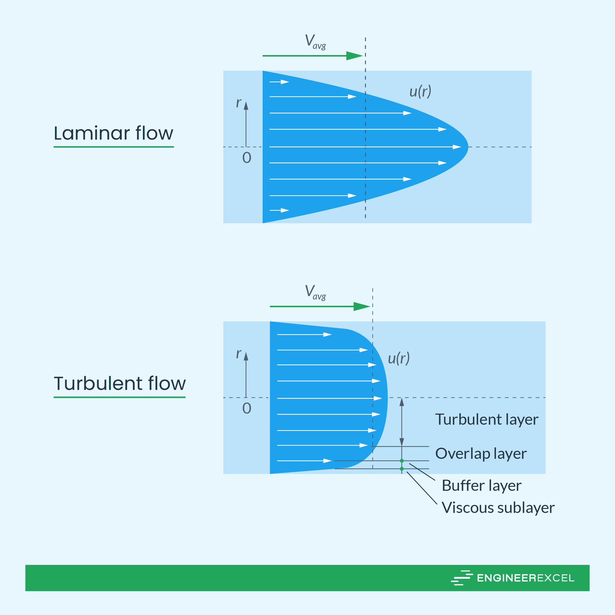
Note that, in laminar flow, the velocity profile across the pipe’s cross-section is parabolic. The maximum velocity occurs at the center of the pipe, gradually decreasing towards the pipe walls. This velocity distribution influences the pressure distribution, with the highest pressure occurring near the pipe walls and the lowest pressure at the center.
Velocity And Pressure Relationship In Turbulent Flow
Turbulent flow is characterized by the presence of eddies, swirls, and vortices, which cause significant mixing and energy dissipation within the fluid. While turbulent flows generally have lower friction factors than laminar flows, they still experience higher pressure losses due to higher fluid velocities. This is because an increase in fluid velocity leads to a squared increase in pressure losses, as evident in the Darcy-Weisbach equation.
In contrast to laminar flow, turbulent flow does not exhibit a parabolic velocity profile, as depicted in the diagram below. Instead, the velocity distribution becomes flatter across the pipe’s cross-section, with increased velocities near the walls. This alteration in velocity distribution leads to a more uniform pressure distribution and reduced pressure variations compared to laminar flow.
Using Velocity And Pressure To Determine Pipe Flow Rate
One of the significant applications of knowing fluid velocity and pressure is measuring pipe flow rate. The process typically involves finding the fluid velocity from the pressure difference between two points first, and then multiplying the fluid velocity with the cross-sectional area to find the volumetric flow rate.
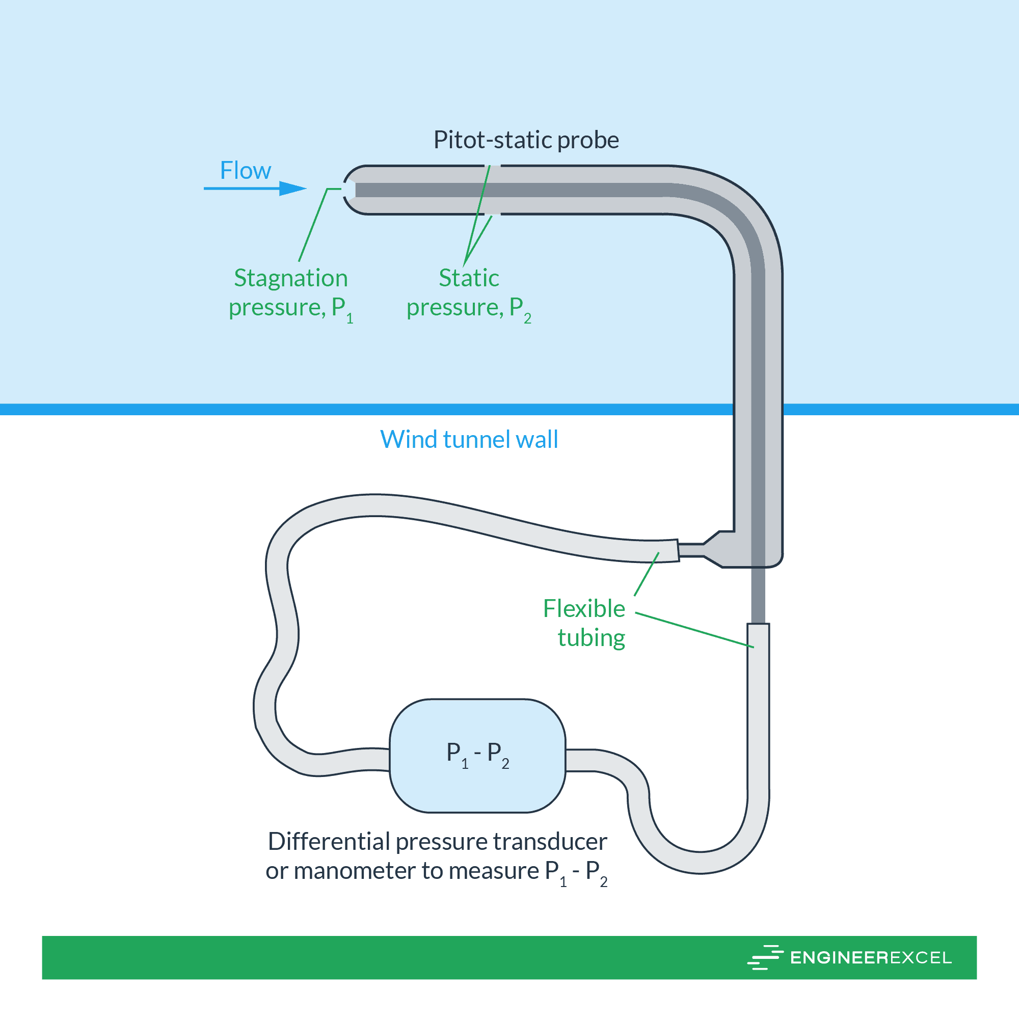
For instance, using a pitot tube, the fluid velocity can be calculated from the difference in stagnation and static pressure using the following formula:
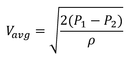
Where:
- P1 = stagnation pressure [Pa]
- P2 = static pressure [Pa]
Once the velocity is obtained, the volumetric flow rate can be calculated by multiplying velocity with the cross-sectional area of the conduit. It is crucial to position the pitot tube accurately at a location where the local velocity matches the average flow velocity and align it properly with the flow to minimize potential errors.
In addition to the pitot tube, there are other flowmeter types that utilize fluid velocity and pressure to estimate the flow rate. Examples include orifice, Venturi, and nozzle meters. These devices are generally referred to as differential pressure flowmeters.