
Understanding the characteristics of different flow patterns is essential for designing efficient fluid systems. In process piping, two often confused flow patterns are plug flow and laminar flow.

This article delves into the differences between these two patterns, examining their distinct flow profiles and practical applications.
Plug Flow vs Laminar Flow
Plug flow and laminar flow both exhibit a streamlined movement of fluid, where distinct layers of the fluid flow parallel to one another. The key distinction between them lies in how their velocity profiles are structured.
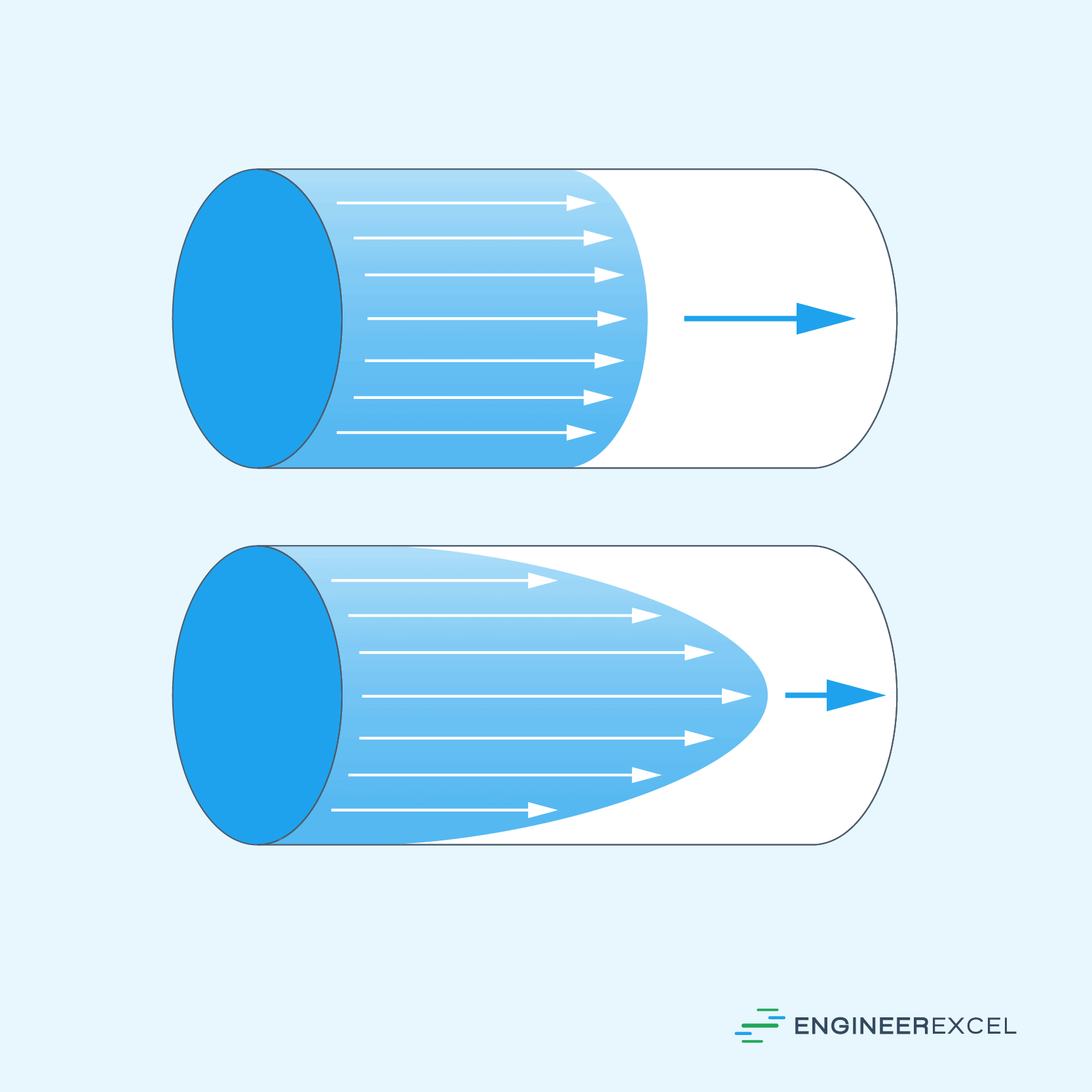
Laminar flow involves varying fluid velocities across the entire cross-section of the conduit due to the no-slip condition at the internal pipe walls and the viscosity of the fluid. As a result, the fluid layer directly adjacent to the wall exhibits zero velocity, while the fluid velocity increases progressively towards the center, forming a parabolic velocity profile.

Elevate Your Engineering With Excel
Advance in Excel with engineering-focused training that equips you with the skills to streamline projects and accelerate your career.
Consequently, the fluid elements in a laminar flow experience different residence time within the conduit. Those situated in the center exit the tube first, while those near the wall exit last.
In contrast, plug flow maintains a flat velocity profile throughout the cross-section. This results in all fluid particles moving at the same speed, akin to a solid plug that moves like a piston inside a cylinder, hence the term. Consequently, all fluid elements travelling through the pipe have an equal residence time.
These flow patterns are illustrated in the diagram below.
Note that plug flow is only an idealization and does not occur in reality exactly as described. Plug flow represents an ideal scenario where there is no boundary layer near the inner pipe wall and the fluid behaves as if it has no viscosity, resulting in zero velocity gradient in the radial direction.
Because all fluid particles move at the same speed, a true plug flow prevents any back mixing. This means that all mixing happens radially, and there is no mixing in the axial direction. In contrast, axial mixing happens in laminar flow.
It is important to clarify that, even though plug flow exhibits a streamlined fluid movement, it is not the same as laminar flow— a common misconception. In reality, plug flow assumes a fully turbulent flow, where the thin laminar layer at the pipe wall becomes insignificant. The thinner this laminar layer, the more closely the flow resembles plug flow.
Plug Flow Reactor
The plug flow model is commonly applied to plug flow reactors, a type of chemical reactor characterized by the continuous flow of reactants through a cylindrical tube in a plug flow pattern.
In a plug flow reactor, reactants enter at one end and flow through the tube at the same velocity, with minimal axial mixing but complete radial mixing. The reactor is typically operated at steady-state, where reactants are continually consumed as they flow down the length of the reactor.
Fluid movement in a plug flow reactor can be modeled as a series of thin “plugs,” each with a uniform and distinct composition. As the flow progresses axially, the concentration within each plug changes, as shown in the diagram below.
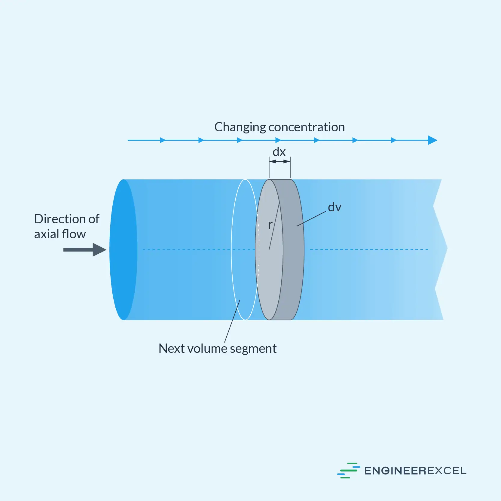
Each plug of differential volume is considered as a separate entity, similar to an infinitesimally small continuous stirred tank reactor. The residence time of each plug is a function of its position in the reactor.
Plug flow reactors are commonly used in applications that require large-scale, continuous production and fast, high-temperature reactions. These include gasoline production, oil cracking, ammonia synthesis, and sulfur dioxide oxidation, among others. In biofuel production, plug flow reactors are also preferred for their steady-state operation without requiring agitation or baffles.
Benefits of Plug Flow
Plug flow offers several advantages. Particularly in chemical reactors, the plug flow model is highly favored due to its continuous and steady operation, ease of control, and high conversion per unit volume. It is also mechanically simple and easy to maintain since there are no moving parts.
With plug flow, thorough mixing occurs radially, eliminating the accumulation of mass gradients of the reactants. This facilitates instantaneous reactant contact, resulting in faster reactions. The reduced reaction time also allows for a more compact plant design.

Moreover, the exceptional radial mixing capability in plug flow allows to uniformly suspend and convey solids along the conduit. This prevents solid buildup, subsequently enhancing the system’s longevity and efficiency.
In terms of modeling and computation, the plug flow model has the advantage that no part of the solution of the problem can be perpetuated upstream. This means that once a plug moves through the system, it does not influence or affect the behavior of the plugs that come after it. This makes it possible to calculate the exact solution to the differential equation knowing only the initial conditions without further iteration.
Among these benefits, however, plug flow reactors suffer from poor temperature control, which can result in undesired thermal gradients.
Plug Flow in Two-Phase Systems
“Plug Flow” can also describe a flow pattern observed in two-phase fluid systems. In these systems, plug flow refers to a specific flow regime where alternating segments of liquid and gas travel along the upper portion of a pipe, while the liquid flows along the bottom of the pipe.
This type of flow occurs when the interface between the liquid and gas is high in the pipe’s cross-section, allowing the waves to gather and make contact with the highest point of the pipe wall. In this case, discrete plugs of liquid alternate with pockets of gas near the upper wall, moving along the axial direction. Gravity-driven flow lines exhibit this particular flow pattern.
In horizontal two-phase pipe systems, plug flow typically happens if the linear velocity of the vapor phase is below 4 ft/s and the liquid phase around 2 ft/s.
Moreover, the pressure drop of the system can be estimated using the Lockhart–Martinelli correlations. These correlations rely on the concept that the pressure drop in a two-phase flow can be calculated by multiplying the pressure drop in a single-phase flow by a factor. This factor is determined under the assumptions that the two-phase flow is both isothermal and turbulent in both the liquid and gas phases, and that the resulting pressure loss is within 10% of the absolute upstream pressure.
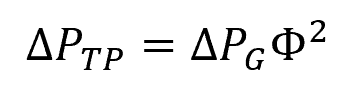
The pressure drop can be calculated using the following equation:
Where:
- ΔPTP = pressure drop for the two-phase plug flow [psi]
- ΔPG = gas phase pressure drop [psi]
- Φ = two-phase flow modulus [unitless]
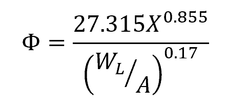
For plug flow, the two-phase flow modulus can be calculated using the following equation:
Where:
- X = Lockhart–Martinelli two-phase flow modulus [unitless]
- WL = liquid flow rate [lb/h]
- A = internal pipe cross-sectional area [ft2]
The Lockhart–Martinelli modulus can be derived using the Darcy relationship as follows:
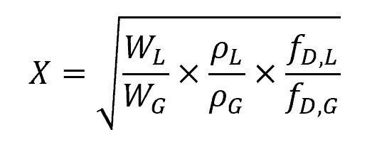
Where:
- WG = gas flow rate [lb/h]
- ρL = liquid density [lb/ft3]
- ρG = gas density [lb/ft3]
- fD,L = Darcy friction factor for liquid phase [unitless]
- fD,G = Darcy friction factor for gas phase [unitless]