
When fluid flows through a pipe, it experiences different types of irreversible losses that cause reduction in fluid energy and pressure. Understanding what these losses are and how they occur is important when designing a piping system, as they directly impact the system’s total head that the pump needs to deliver.

This article explores the different types of losses that occur in pipe flow and the associated calculations.
Different Types of Losses in Pipe Flow
Before discussing the different types of losses in pipe flow, it is important to first understand what is meant by losses. In fluid mechanics, losses in pipe flow can refer to both energy losses and pressure losses, and these terms are often used interchangeably.
When pressure losses occur in a pipe, it is because some of the fluid’s energy is being converted into other forms, such as heat or noise. In designing piping systems, however, the primary concern lies with pressure losses, as they directly influence the pumping power requirement of the system.

Elevate Your Engineering With Excel
Advance in Excel with engineering-focused training that equips you with the skills to streamline projects and accelerate your career.
Pressure losses can stem from multiple factors. Most texts categorize them into two types: major losses, resulting from friction, and minor losses, associated with changes in flow direction or cross-sectional area of the conduit. However, these classifications only address mechanical energy losses in piping systems.
In reality, there are other factors that contribute to losses in pipe flow, including those related to heat transfer and electromagnetic fields. These will be discussed in the following sections.
Major Losses in Pipe Flow
Major losses are caused by the friction between the fluid and the pipe wall. These losses are influenced by several factors, including the viscosity of the fluid, the surface roughness of the pipe’s internal wall, the velocity of the flow, and the length of the pipe. In a typical system with long pipes, these friction-induced losses constitute the majority of the total head loss, hence the term ‘major losses.’
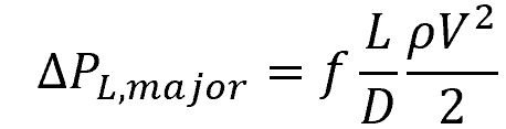
To calculate major losses resulting from friction, the Darcy-Weisbach equation can be used:
Where:
- ΔPL, major = pressure loss due to friction [Pa]
- f = Darcy friction factor [unitless]
- L = length of pipe [m]
- D = hydraulic diameter of pipe [m]
- ρ = density of the fluid [kg/m3]
- V = average fluid velocity [m/s]
This equation is applicable for all types of fully developed internal flows, including laminar or turbulent flows, circular or noncircular pipes, smooth or rough surfaces, and horizontal or inclined pipes.
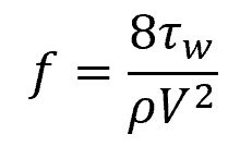
The Darcy friction factor is a dimensionless parameter that characterizes the frictional resistance of the fluid flow. It can be mathematically defined as:
Where:
- τw = shear stress at the pipe wall [Pa]
In general, the value of the Darcy friction factor depends on the Reynolds number and the relative roughness of the pipe surface. There are several ways to determine this value for a given pipe flow. One of them is to use the Moody chart, shown below:
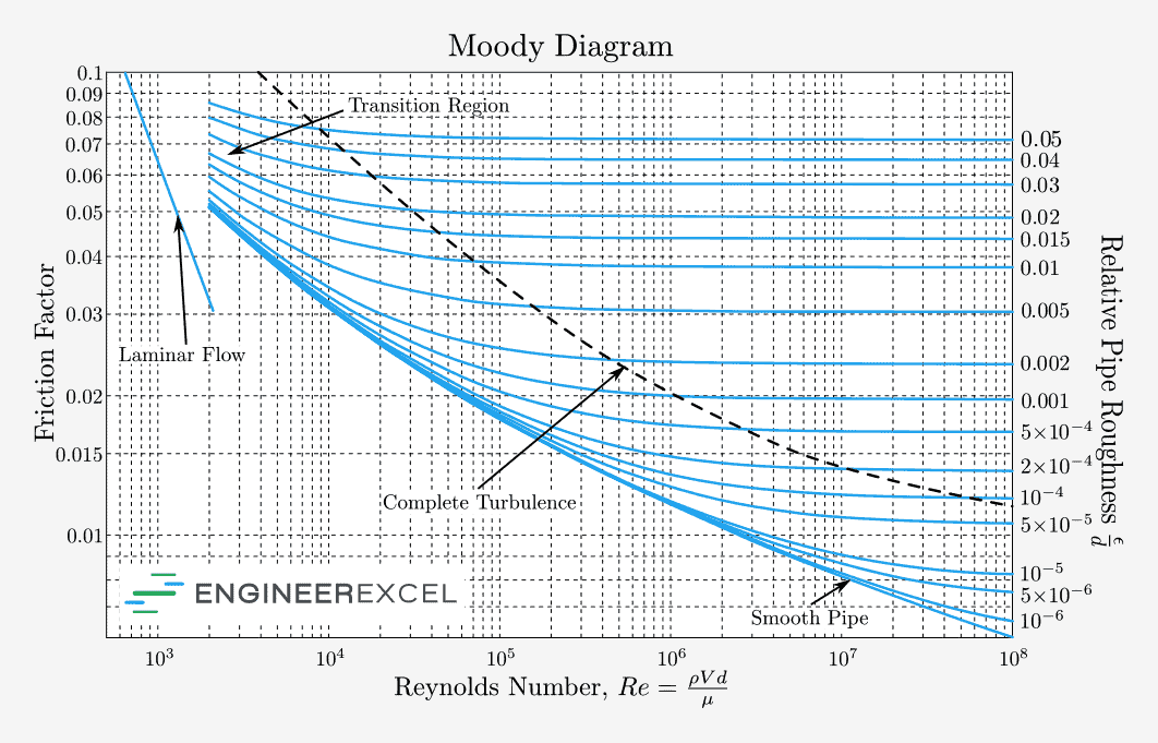
The Moody chart plots the relationship between friction factor (f), Reynolds number (Re), and relative pipe roughness (ε/D).
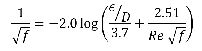
Another way to determine the Darcy friction factor is to use empirical formulas. One of them is the Colebrook equation, which is the basis of the Moody chart and is widely accepted as the design formula for turbulent friction. It can be written as follows:
Where:
- ε = average height of surface irregularities on the internal pipe wall [mm]
- D = pipe diameter [mm]
- Re = Reynolds number [unitless]
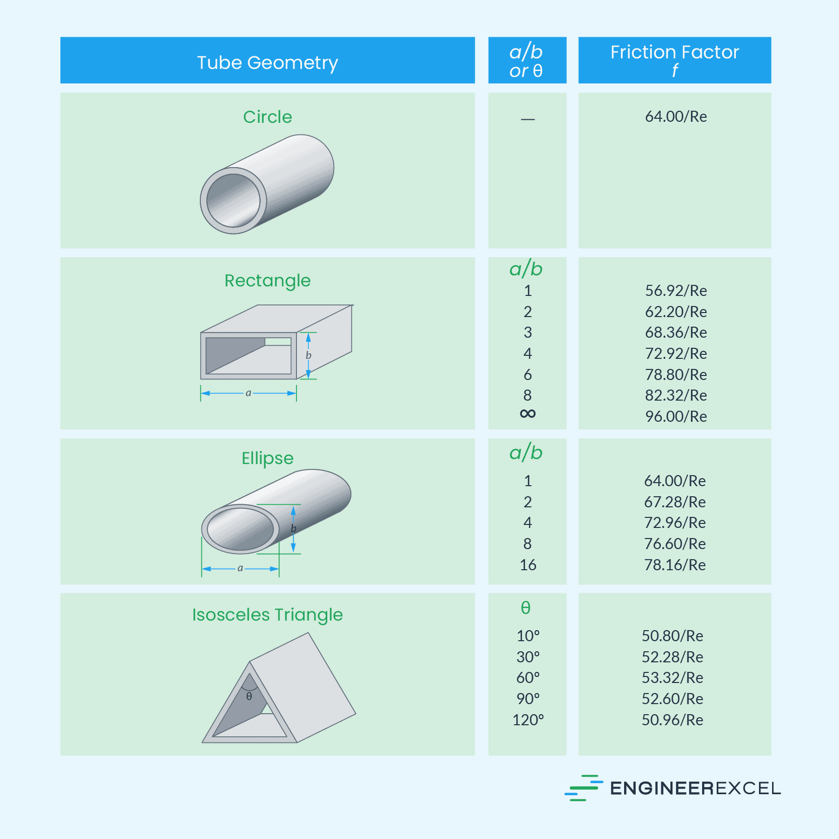
For laminar flow, the formula for the friction factor in pipes of different cross sections are tabulated in the diagram below:
In practice, it is common to express pressure losses in terms of the head loss. The head loss represents the equivalent height that the fluid needs to be raised by a pump in order to overcome the frictional losses in the pipe.
To calculate for the major head loss, the Darcy-Weisbach equation can be transformed as follows:
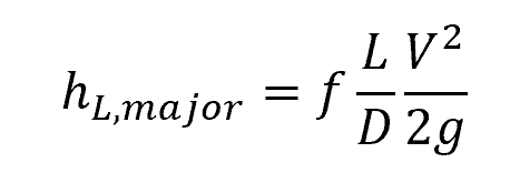
Where:
- hL, major = head loss [m]
Minor Losses in Pipe Flow
A typical piping system comprises not only straight pipes but also various components such as fittings, valves, bends, elbows, tees, inlets, outlets, expansions, and contractions. These components disrupt the smooth flow of the fluid, leading to additional losses as they cause separation and mixing of the fluid flow. These losses are commonly referred to as minor losses.

In systems with long pipes, these losses are typically small compared to the total head loss, which is why they are termed “minor losses.” However, it is important to note that in certain cases, minor losses can outweigh major losses in magnitude. This can occur when there are multiple turns and valves in a short distance, or when a valve is partially closed, significantly increasing the head loss.
The flow through valves and fittings is highly complex, making theoretical analysis impractical. Hence, determining minor losses is primarily done through experimental methods.
The minor loss caused by a specific component can be quantified using a dimensionless parameter called the loss coefficient, which is defined by the following equation:
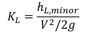
Where:
- KL = loss coefficient caused by the insertion of a component [unitless]
- hL, minor = head loss caused by the component [m]
The value of the loss coefficient generally depends on the geometry of the component and the Reynolds number. However, to simplify the analysis, it is usually assumed to be independent of the Reynolds number. This is an acceptable simplification since most flows occur at the turbulent flow regime where the value of loss coefficients tends to be independent of the Reynolds number.
As shown in the diagram below, the minor loss caused by inserting a specific component into a pipe section is obtained by measuring the difference in pressure loss across the pipe section with and without the component.
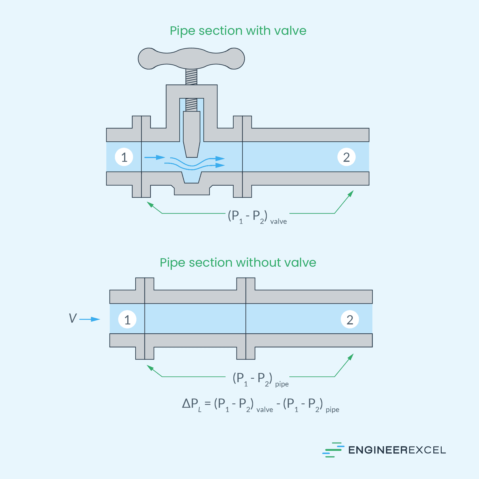
It is essential to emphasize that when measuring the minor loss attributed to a component, the pressure difference should be measured between the upstream side of the component and a location considerably downstream, typically tens of pipe diameters away. This ensures a complete assessment of the component’s overall impact on the head loss. While most of the irreversible head loss happens close to the component, some of it extends downstream because of the induced turbulent eddies that continue to dissipate mechanical energy as the fluid flows through the pipe.
Manufacturers typically determine the loss coefficients of components through experiments. Nevertheless, there are also published values available for common components, such as inlets, exits,
bends, sudden and gradual area changes, and valves.
Although with significant uncertainty, these values can be employed for initial calculations. However, it is strongly recommended to use actual manufacturer’s data for a more accurate calculation.
Loss Coefficient for Pipe Flow Entry
The loss coefficient for pipe flow entry is significantly influenced by geometry. As depicted in the diagram below, well-rounded inlets exhibit lower head loss compared to sharp-edged inlets. This is because the fluid cannot make sharp turns easily, resulting in flow separation at the corners.

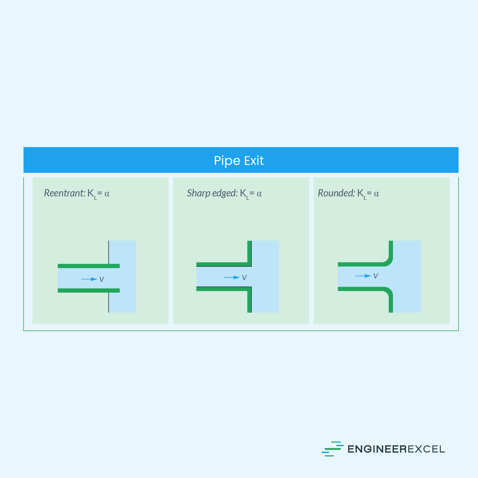
Loss Coefficient for Pipe Flow Exit
The loss coefficient for a submerged pipe exit is equal to the kinetic energy correction factor, which is about 1 for fully developed turbulent pipe flow and around 2 for fully developed laminar pipe flow. This is because, when fluid exits a submerged pipe, it loses all its kinetic energy as it mixes with the reservoir fluid and eventually comes to rest due to the action of viscosity. This is true for any exit geometry.
Loss Coefficient for Sudden Expansion
Piping systems often involve changes in the conduit’s cross-sectional area in order to accommodate variations in flow rate, velocity, or density of the fluid.

For a sudden pipe expansion, the loss coefficient can be calculated using the following formula:
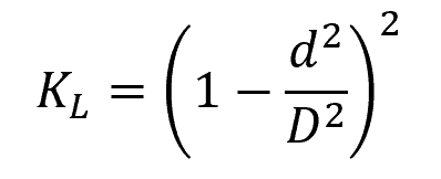
Where:
- d = diameter of the smaller pipe [m]
- D = diameter of the larger pipe [m]
Note that this loss coefficient is based on the velocity in the smaller-diameter pipe.
Loss Coefficient for Sudden Contraction
For a sudden pipe contraction, the loss coefficient can be approximated using the graph below.
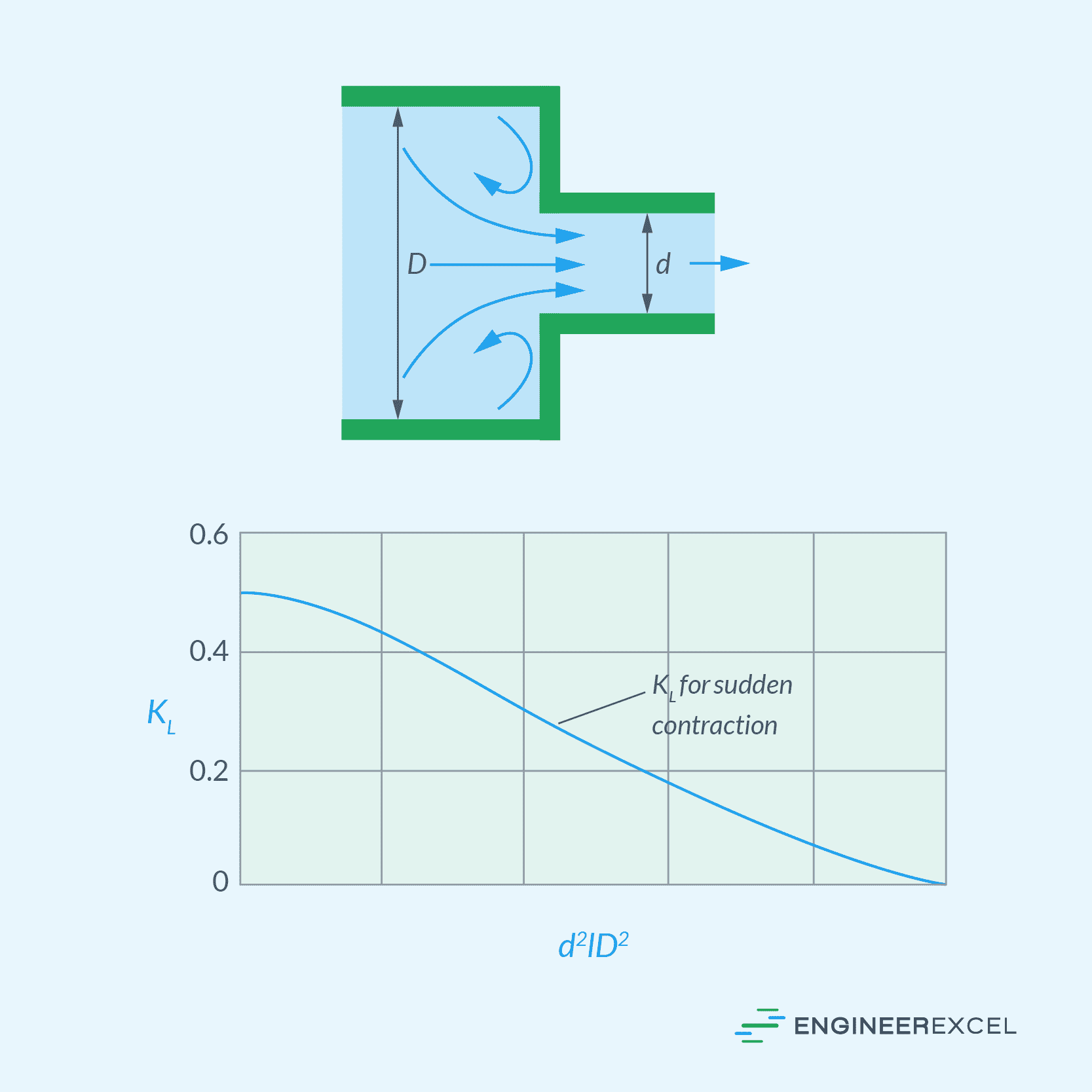
These loss coefficient values are also based on fluid velocity in the smaller-diameter pipe.
Loss Coefficient for Bends and Branches
The diagram below shows loss coefficients for typical configurations of bends and branches. Notice that these values are not only dependent on the angle and smoothness of the bends, but also on the type of connection— whether flanged or threaded.

Loss Coefficient for Valves
A valve regulates head loss by adjusting its opening until the desired flow rate is attained. Ideally, valves should exhibit minimal loss coefficients when fully open to minimize head loss during full-load operation.
Below are the typical loss coefficients for various types of valves:
| Globe valve, fully open: K(L) = 10 | Gate valve, fully open: K(L) = 0.2 |
| Angle valve, fully open: K(L) =5 | Gate valve, ¼ closed: K(L) = 0.3 |
| Ball valve, fully open: K(L) = 0.05 | Gate valve, ¼ closed: K(L) = 2.1 |
| Swing check valve: K(L) = 2 | Gate valve, ¼ closed: K(L) = 17 |
Notice that the loss coefficient increases drastically as a valve is closed
Thermal Losses in Pipe Flow
Major and minor losses account for the mechanical energy dissipation in pipe flow. However, when dealing with flows involving heat transfer, it becomes essential to consider thermal losses. These normally happen when there is a temperature difference between the fluid and the pipe wall.
Thermal losses can arise due to multiple heat transfer processes, including conduction, convection, and radiation. These losses manifest both within the fluid itself and at the interface between the fluid and the pipe wall.
Electromagnetic Losses in Pipe Flow
When a conducting fluid flows through a pipe and is subjected to a magnetic field, it can experience a phenomenon called magnetohydrodynamic (MHD) drag. This drag occurs due to the interaction between the magnetic field and the electric currents induced within the fluid. As a result, additional forces are exerted on the fluid, which can lead to pressure losses.
In a study conducted by Malekzadeh et al. involving laminar pipe flows, it was observed that the pressure drop is directly proportional to the square of the magnetic field’s strength multiplied by the sine of the magnetic field angle.
Total Head Loss Calculation
After identifying all the different types of losses within a piping system, the total head loss of the system is calculated by summing these individual losses:

Where:
- hL, total = total head loss [m]
- hL, thermal = thermal head loss [m]
- hL, electromagnetic = electromagnetic head loss [m]
Once the total head loss of the system is known, the required pumping power to overcome the pressure loss can be calculated using the following equation:
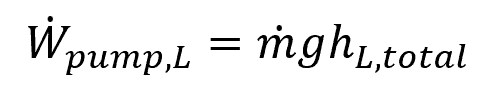
Where:
- Wpump, L = required pumping power to overcome pressure losses [W]
- m = mass flow rate [kg/s]
- g = gravitational acceleration [9.81 m/s2]