
In this post, you’ll learn how to create a catenary cable tension calculator in Excel by solving an implicit equation. The example will show specifically how to use Goal Seek for finding roots of equations in Excel.
Video
Subscribe to EngineerExcel on YouTube
Catenary Cable Tension Calculator in Excel – Finding the Root of an Implicit Equation
Catenary Cable Background
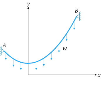
A catenary cable is a cable hung between two points that are separated horizontally by some distance. The only load acting on the cable is its own weight:

Elevate Your Engineering With Excel
Advance in Excel with engineering-focused training that equips you with the skills to streamline projects and accelerate your career.
The image below shows a free body diagram of a section of the cable. At the lowest point of the cable, the tension force is horizontal.
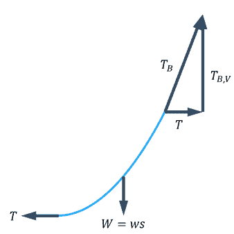
And the tension at the lowest point is related to the geometry of the cable by this equation:
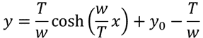
where
- T is the horizontal component of tension
- W is the weight of the cable per unit length
- y0 is the height of the lowest point of the cable measured from some reference
- x and y are points that the cable passes through measured from that same reference.
Solving for Catenary Cable Tension in Excel
If the geometry and mass properties of the cable are known, this equation could be solved for the tension.
However, that’s difficult because T is an implicit variable, and the equation cannot be rearranged to put T alone on one side of the equal sign.
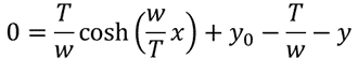
Instead, root finding can be used to calculate the tension. In root finding the equation is rearranged so zero is alone on one side of the equation.
Then an iterative method is used to find the value of T that causes the right side of the equation to be equal to zero.
How to Calculate Catenary Cable Tension in Excel
The quickest way to find roots in Excel is to use Goal Seek. The steps to find the roots of the above equation, and thereby the tension at the low point in the cable are below. The spreadsheet has already been set up to store the inputs and the outputs.
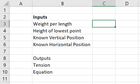
Step 1: Enter the Input Values for the Catenary Cable Calculation
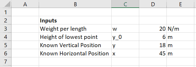
There are four inputs to the problem:
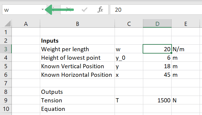
- The weight per unit length, w, has a value of 20 N/m
- The height of the lowest point in the cable, y_0, has a value of 6 meters
- The known vertical position, y, is 18 meters
- The known horizontal position, x, is 45 meters.
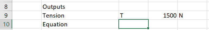
Step 2: Enter a Guess Value for the Cable Tension
Tension is technically an output but is entered as a value in the spreadsheet. In a subsequent step, Goal Seek will be used to automatically iterate through values of T to find the correct value.
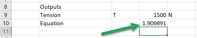
Call this value T and enter an initial guess value of 1500 Newtons.
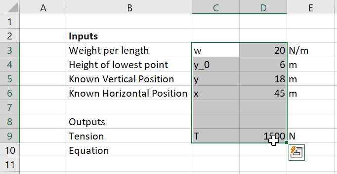
Step 3: Create Names for the Variables in the Catenary Cable Equation (Optional)
Excel equations are much easier to read and understand when names are assigned to cells that will be included in the formula. This step is completely optional but can be a huge benefit.
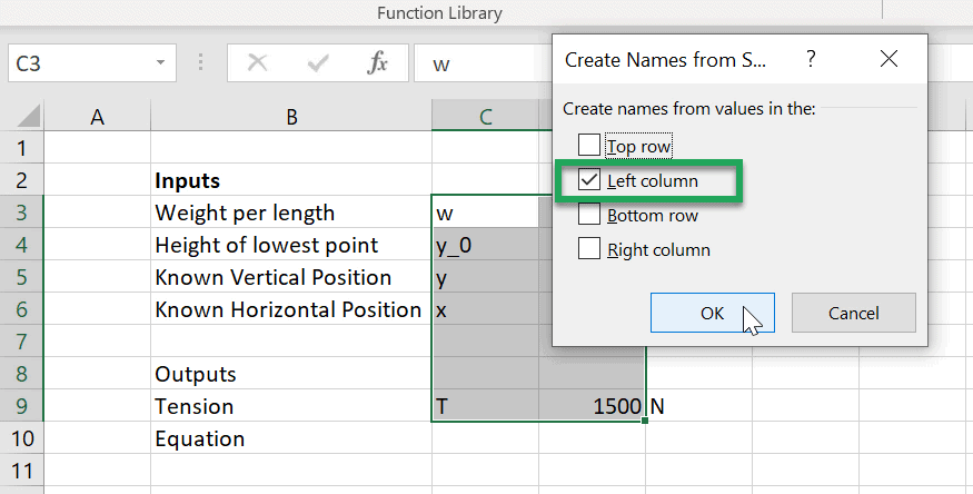
To create names for the catenary cable inputs, select all the cells containing the variable names and values. (It’s ok if some extra blank cells are also selected.)
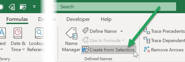
Next, navigate to the Formulas tab and select “Create from Selection“.
In the window that opens, make sure that the left column box is selected. Once it is selected, click okay.
Now each of the cells has been assigned a name corresponding to the variable name entered in the cell to the left. Clicking each cell reveals the name in the Name Box in the upper left of the Excel window.
Step 4: Enter the Formula for the Catenary Cable
With names applied to the cells, it is much easier to type the formula for the cable by calling the cells by name.
The formula includes the COSH function, which returns the hyperbolic cosine of an argument in Excel.
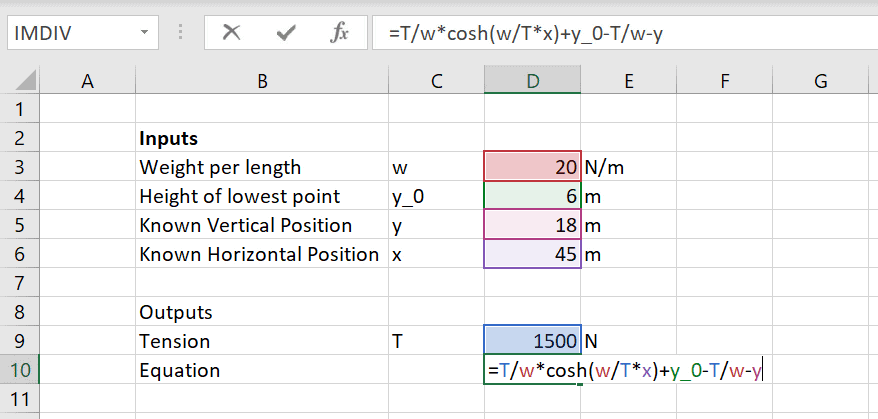
Because the Tension value entered in Cell D9 is just a guess, the result of the formula is not zero. In other words, it is not a root of the equation.
Step 5: Open the Goal Seek Tool
Goal Seek can start from the initial guess value and iterate to find a value of T that will make the result of the formula equal to zero.
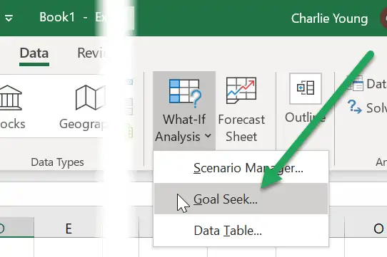
To open the Goal Seek tool:
- Open the Data tab
- Click What-If Analysis
- Select “Goal Seek”
Step 6: Set up Goal Seek to Find the Tension in the Cable
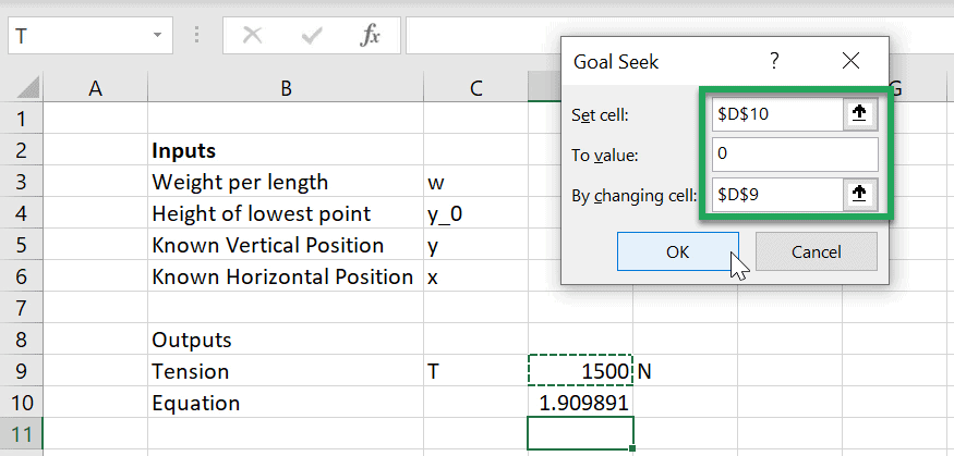
Once Goal Seek has opened, set it up to iterate on the value of tension until the equation is equal to 0.
- Change the “Set Cell” to cell D10 (or the cell containing the formula).
- Enter a value of “0” in the “To value:” field.
- Finally, select D9 (or the cell containing the value of cable tension) for the field “By changing cell:”
Step 7: Run Goal Seek to Calculate the Catenary Cable Tension in Excel
Once all those fields have been filled out, click OK. Goal Seek should find a solution within seconds, often in less than a second.
Results
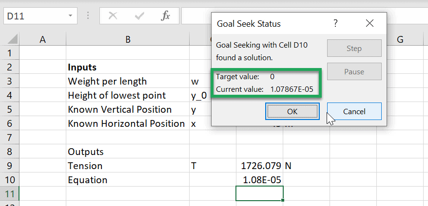
In this example, Goal Seek achieves a value of 1.08×10^-5, which is essentially zero plus a negligible amount of error. The resulting tension is 1726 Newtons.
Of course, keep in mind that if any of the values in the “Inputs” section change, Goal Seek must be run again. However, it is possible to automate Goal Seek so that it runs whenever a change occurs on the spreadsheet, as explained in this post.
Related Topics
- Named Cells
- Trigonometry Functions in Excel
- Using Goal Seek to Solve the Colebrook Equation in Excel