There are several ways to find the roots of equations in Excel. The most basic way is to do so graphically, using a scatter chart.
In this example, we’ll try to find the root of the Colebrook equation. This equation is used to find the Darcy Weisbach friction factor for flow in a pipe without having to look it up on a Moody chart.

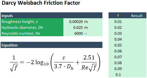
The inputs to the equation are the Reynolds number (Re), the hydraulic diameter (Dh), and the wall roughness (ε).
The problem with this equation is that it is implicit. If you want to solve for the friction factor, f, there is no way to arrange the equation such that f is on one side, and all the other variables are on the other.

Elevate Your Engineering With Excel
Advance in Excel with engineering-focused training that equips you with the skills to streamline projects and accelerate your career.
Luckily, we can use Excel to find the solution using a few different methods. I’ll demonstrate in this post how to find the root of the equation graphically.
If we rearrange this equation so that everything is on one side of the equal sign, the friction factor value that causes that equation to be equal to zero must be the solution.

Given some input values for Re, Dh, and ε, we can enter a range of guesses for f, and calculate the left side of the equation above.
To start, enter values of 0.01 and 0.02 in the column for f. Select these cells, then drag the fill handle down. This will fill in values for f from 0.01 – 0.1:

Select the f values, then name the array f using the name box to the left of the formula bar. The other variables have already been assigned names: eps for the roughness, DH for the hydraulic diameter, and Re for the Reynolds number. We can use these variable names in an array formula. In the top cell of the result column, enter the formula:
=1/SQRT(f)+2*LOG10(eps/(3.7*DH)+2.51/(Re*SQRT(f)))
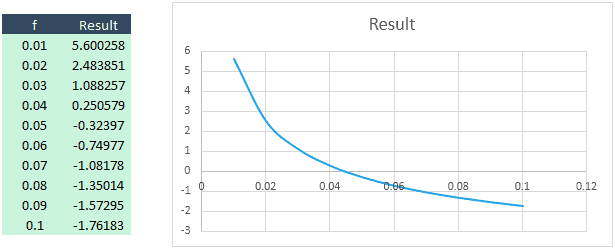
Use Ctrl-Shift-Enter to enter the formula so it will be applied to the entire array. Select all the data and insert an XY scatter chart to display the data. The results in the spreadsheet tell us that the value of “f” is somewhere within this range because the numbers change from positive to negative. The chart makes it even easier to see that the line crosses zero somewhere between 0.04 and 0.05:

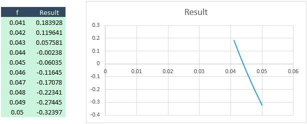
We can use increasingly granular guesses for f to identify the solution to the equation. Erase the values for f, and enter 0.041 in the first box. In the second box, enter 0.042. Select those cells and double-click the fill handle to complete the table.

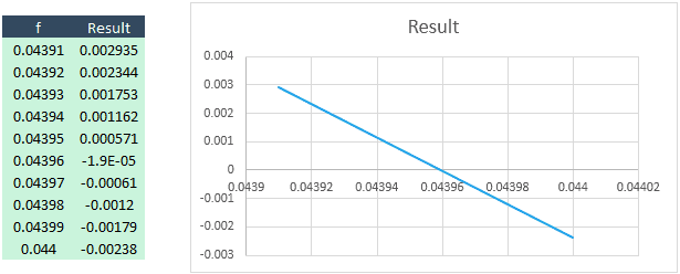
From the data at left, we can see that the line crosses zero somewhere between f = 0.043 and f = 0.044. Enter a new range starting with 0.0431 and 0.0432, using the fill handle to complete the table. The data then show that the line crosses zero somewhere between 0.0439 and 0.044. For the next round, use 0.04391 as the initial guess value and 0.04392 as the next. Fill the rest of the column.

It’s clear on the chart that the line crosses at 0.04396. If we examine the data table, the error on that value is -1.9 x 10⁻⁵, which is quite small. This is good accuracy, so we can stop here.
You may have noticed that you could have done this exercise without the chart by examining the values in the table. The chart is optional, but it’s fast to add one, and it gives you a visual that you can interpret with a quick glance.
