
In fluid mechanics, one of the simplest models used as an example to understand the behavior of fluids in motion is laminar flow over a flat plate. This is characterized by a viscous fluid flowing over a flat surface in a smooth and orderly manner.

This article explores the characteristics of laminar flow over a flat plate, particularly the formation of its boundary layer.
Laminar Flow Over Flat Plate
Laminar flow is characterized by the smooth and orderly movement of fluid particles along parallel layers or streamlines with little or no mixing between adjacent layers. In fluid mechanics, one of the most widely studied cases of laminar flow involves the flow of fluid over a flat plate. This type of flow finds applications in various fields, including the study of plate heat exchangers, aerodynamic surfaces in vehicles, surface coating processes, and microfluidics.
When fluid flows over a flat plate, the fluid adjacent to the surface is affected by the interactions between the fluid particles and the surface. This creates a region of disturbed flow called the boundary layer, where the effect of viscous forces is felt.

Elevate Your Engineering With Excel
Advance in Excel with engineering-focused training that equips you with the skills to streamline projects and accelerate your career.
This boundary layer is essentially a thin layer of fluid adjacent to the surface, characterized by a rapid change in fluid properties as it moves away from the surface. From the leading edge of the plate, the thickness of the boundary layer increases until it reaches a specific point called the entrance length. At this point, the boundary layer stops growing, and a fully developed flow starts to form.
Two types of boundary layers are commonly analyzed in this context: the hydrodynamic boundary layer, which is related to the velocity profile, and the thermal boundary layer, which is linked to the temperature profile.
Hydrodynamic Boundary Layer in Laminar Flow Over Flat Plate
When a fluid flows over a flat plate, the fluid in direct contact with the surface adheres to it due to the no-slip condition. This means that at the surface itself, the fluid velocity is zero.
As the distance from the solid surface increases, the velocity of the fluid also increases. This transition region, where the velocity gradually changes from zero to the free-stream velocity, is called the hydrodynamic boundary layer. Outside this layer, the flow behaves more like an ideal fluid with constant free-stream velocity, and viscous effects are negligible.
To illustrate, consider the diagram below.
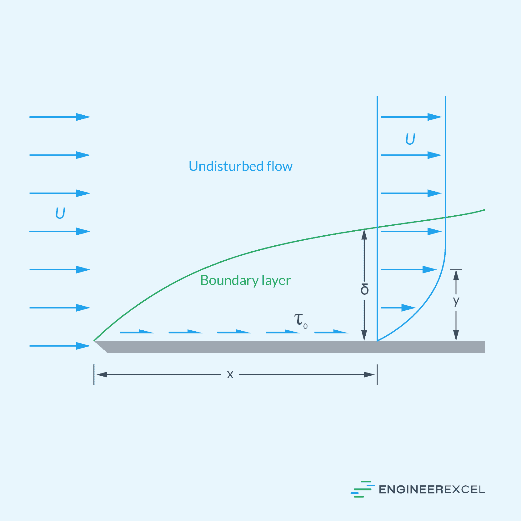
Within the hydrodynamic boundary layer, the velocity gradients are significant, and viscous effects dominate. Due to the exchange of momentum between fluid molecules, there is a net movement of momentum from high-velocity to low-velocity regions, resulting in a force along the direction of the flow.
This force is due to the shear stress caused by the viscosity of the fluid, which can be calculated using the following formula:
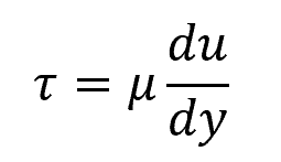
Where:
- τ = shear stress [Pa]
- μ = dynamic viscosity of the fluid [N-s/m2]
- u = fluid velocity [m/s]
- y = perpendicular distance of the fluid layer from the plate [m]
Thickness of Hydrodynamic Boundary Layer for Laminar Flow Over Flat Plate
The thickness of the hydrodynamic boundary layer is defined as the distance from the plate to the point where the fluid velocity is 99% of the free-stream velocity. As shown in the diagram above, this thickness starts very thin at the entrance and gradually thickens as it moves across the plate.
It is important to note that the boundary layer technically does not start at the very edge of a flat plate. At the leading tip, there is a region, called the stagnation point, where the fluid particles are brought to a standstill before they start to flow along the surface of the plate. Because of this, the boundary layer starts to form a few distance upstream.
However, this distance is often neglected to simplify analysis; especially at higher velocities, where its value becomes very small. For a smooth flat plate, the thickness of the hydrodynamic boundary layer can be approximated using the following formula:
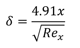
Where:
- δ = thickness of the boundary layer [m]
- x = distance from the leading edge of the plate [m]
- Rex = local Reynolds number [unitless]
In general, the thickness of the boundary layer becomes thinner at higher fluid velocities.
Reynolds Number for Laminar Flow Over Flat Plate
The local Reynolds number characterizes the local flow regime with respect to the distance from the leading edge of the plate. Its value increases linearly downstream and can be calculated using the following formula:
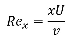
Where:
- U = free-stream fluid velocity [m/s]
- v = kinematic viscosity [m2/s]
If undisturbed, the laminar boundary layer will remain laminar up to a local Reynolds number value of approximately 500,000. After this, the flow transitions to become turbulent. Although this critical Reynolds value is true for most analytical purposes, its true value is highly dependent on the roughness of the flat plate’s surface and the flow conditions on the free-stream region.
Shear Stress for Laminar Flow Over Flat Plate
The local Reynolds number also affects the value of the shear stress at the plate. For an incompressible flow along a smooth plate, this can be calculated using the following formula:
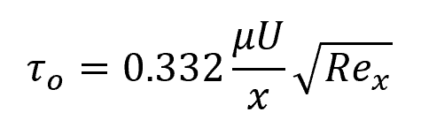
- τo = shear stress at the plate [Pa]
Thermal Boundary Layer in Laminar Flow Over Flat Plate
Just as there is a hydrodynamic boundary layer where velocity gradients are formed due to the effects of viscosity, there is also a thermal boundary layer where temperature gradients are formed when heat is transferred from the flat plate to the fluid or vice versa. This occurs if there is a difference between the bulk temperature of the fluid and the surface temperature of the flat plate, resulting in net heat movement perpendicular to the direction of the flow.
To illustrate, consider the diagram below showing the formation of the thermal boundary layer of a laminar flow over a flat plate with a surface temperature of Tw and a free-stream temperature of T∞.
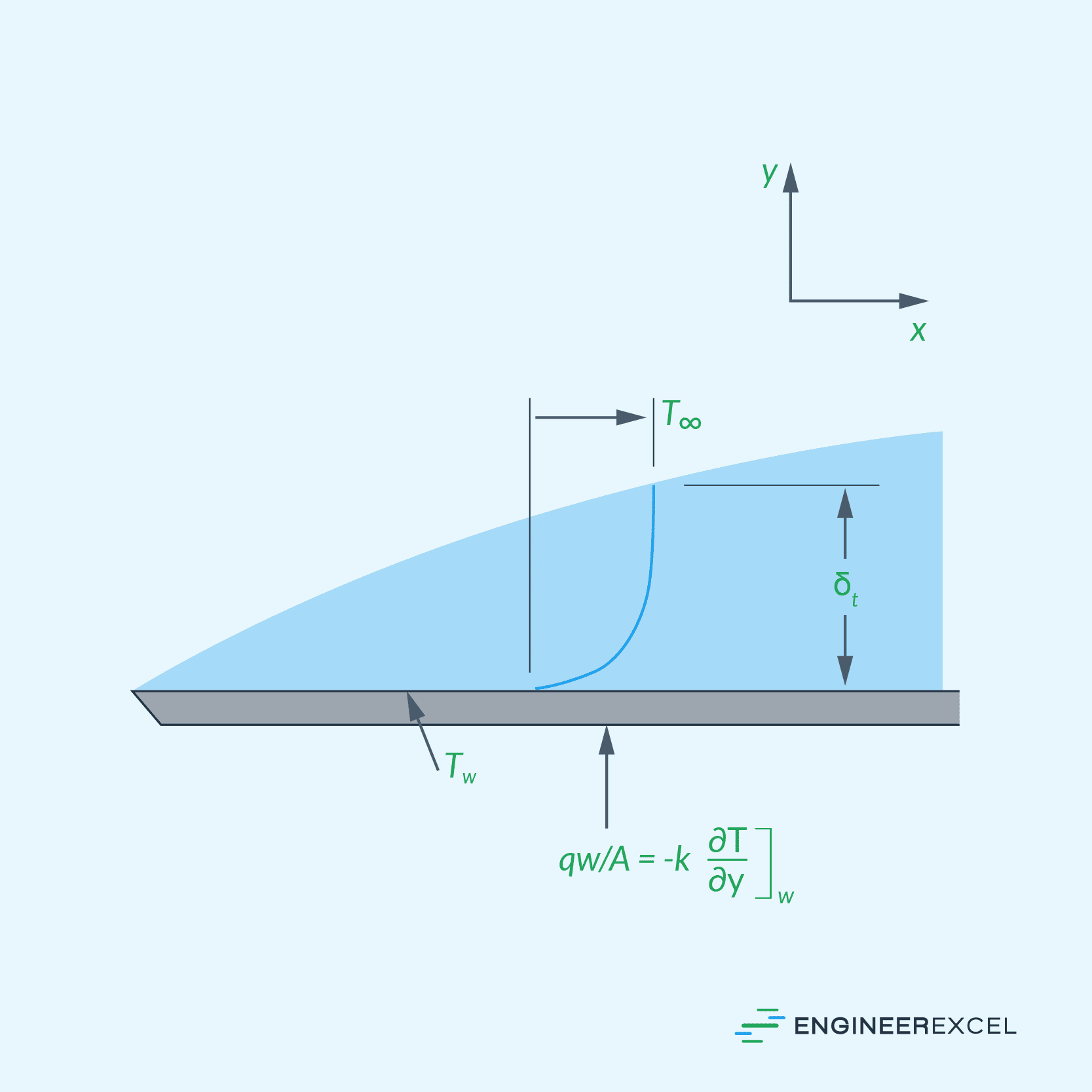
Within the thermal boundary layer, the fluid temperature changes rapidly from the surface temperature of the plate to the free stream temperature away from the plate. Beyond this layer, the fluid is assumed to have a constant bulk temperature.
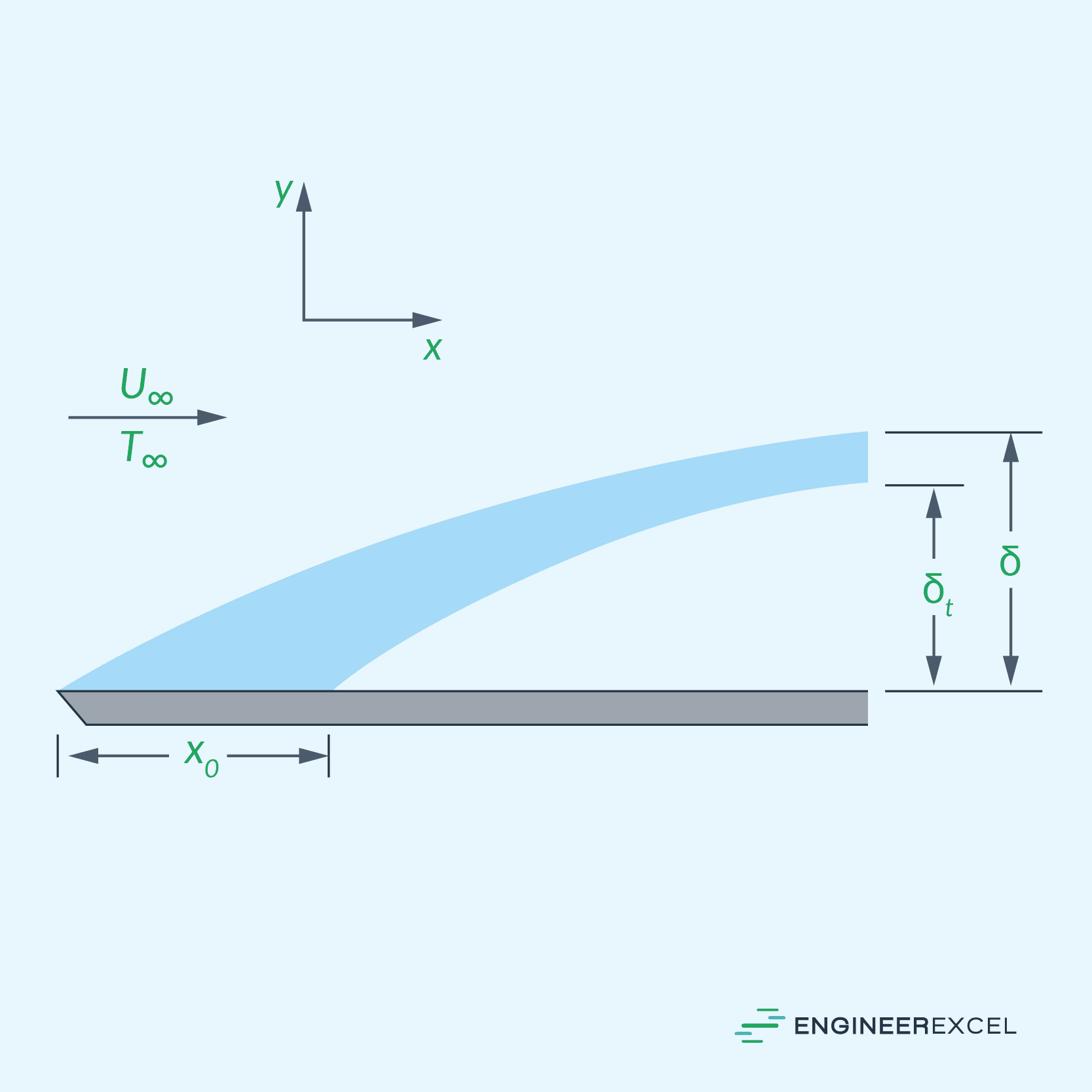
Thickness of Thermal Boundary Layer for Laminar Flow Over Flat Plate
The thickness of the thermal boundary layer is defined as the perpendicular distance from the plate to a point where the flow temperature has reached 99% of the free stream temperature. Just like the hydrodynamic boundary layer, the thickness of the thermal boundary layer starts thin at the leading edge and increases as the fluid flows across the plate. However, it is important to note that these boundary layers typically differ in size.
The thickness of the hydrodynamic boundary layer depends primarily on fluid viscosity, whereas the thickness of the thermal boundary layer is primarily influenced by the fluid’s thermal diffusivity.
For laminar flow over a flat plate, the following equation can be used to describe the relationship between the thickness of the hydrodynamic boundary layer and the thickness of the thermal boundary layer:
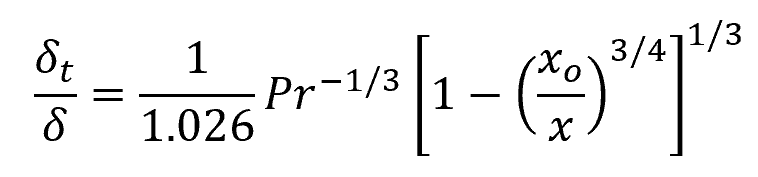
Where:
- δt = thickness of the thermal boundary layer [m]
- Pr = Prandtl number [unitless]
- x = distance from the leading edge of the plate [m]
- xo = start of heating of the plate [m]
If the plate is heated over its entire length, such that the value of xo is zero, the above formula can be simplified as follows:
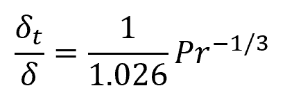
This formula is applicable for cases in which the thermal boundary layer is thinner than the hydrodynamic boundary layer— a condition that holds true for the majority of gases and liquids. This assumption is generally valid for fluids with a Prandtl number greater than 0.7. However, it is important to note that there are exceptions, such as liquid metals which have Prandtl numbers on the order of 0.01.
The Prandtl number is a dimensionless number that measures the relative magnitude between the momentum diffusion caused by viscous effects and the thermal diffusion within a fluid. It can be mathematically expressed as follows:
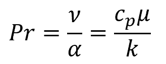
Where:
- α = thermal diffusivity [m2/s]
- cp = specific heat capacity [J/kg-K]
- k = thermal conductivity [W/m-K]
Nusselt Number for Laminar Flow Over Flat Plate
The Nusselt number is a dimensionless number defined as the ratio of convective heat transfer to conductive heat transfer. In other words, it quantifies the enhancement of heat transfer within the fluid due to convection compared to pure conduction. It is typically expressed as:
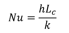
Where:
- Nu = Nusselt number [unitless]
- h = convective heat transfer coefficient [W/m2-K]
- Lc = characteristic length of the flow [m]
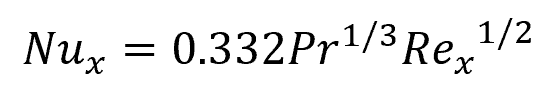
For laminar flow over a flat plate, obtaining the Nusselt number depends whether the plate is heated at constant temperature or at constant heat flux. For an isothermal flat plate, the local Nusselt number with respect to the distance from the leading edge of the plate can be obtained using the following empirical formula:
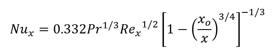
Where:
- Nux = local Nusselt number [unitless]
If the plate is heated over its entire length, such that the value of xo is zero, the above formula can be simplified as follows:
On the other hand, if the plate is heated at constant heat flux, the formula for the local Nusselt number becomes:

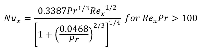
The above formulas are applicable for fluids having Prandtl numbers between about 0.6 and 50. For fluids outside this range, e.g., liquid metals and heavy oils, the following empirical formula by Churchill and Ozoe can be used to calculate for the local Nusselt number in laminar flow on an isothermal flat plate:
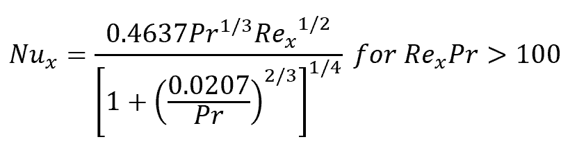
In the case of a constant heat flux, the same form of the formula can be used but with different coefficients:
Applications and Examples of Laminar Flow Over Flat Plate
Understanding laminar boundary layers over flat plates has numerous practical applications across various industries. For instance, in heating and cooling industries, the flat plate model can be used for designing and analyzing the performance of plate heat exchangers. In these applications, precise control of the boundary layer is important to achieving optimal heat transfer efficiency.
In the aerospace industry, the same model can be used in designing efficient wing profiles. By manipulating the boundary layer, the onset of turbulence can be delayed, which reduces drag and enhances aircraft fuel efficiency. Similarly, this concept extends to land vehicle design, where it can be applied to optimize aerodynamics and improve vehicle performance.