
Gradually varied flow refers to the gradual change in water surface elevation along an open channel, typically occurring in reaches with varying channel slopes and cross-sectional shapes. This phenomenon is governed by the balance between gravity, frictional resistance, and centrifugal forces, leading to a smooth transition of flow properties along the channel.
In this article, we will discuss the characteristics of gradually varied flow, its equation, and the different channel slope classifications.
What is Gradually Varied Flow
The most common way to classify open-channel flows is by the rate of change of the free-surface depth. When the depth remains constant, it’s called uniform flow. If the depth changes, the flow is considered varied.
Varied flows typically happen if there are changes in the channel slope or cross-section, or if there’s an obstruction in the flow. If the change in depth is gradual, then it is said to be a gradually varied flow.

Elevate Your Engineering With Excel
Advance in Excel with engineering-focused training that equips you with the skills to streamline projects and accelerate your career.
A gradually varied flow is a steady non-uniform flow that occurs in open channels when there is a gradual change in the channel’s bottom slope, cross-sectional shape, or an obstruction in the path that affects the flow depth and velocity. Unlike rapidly varied flow, changes in gradually varied flow take place over long distances, allowing friction to act on the flow.
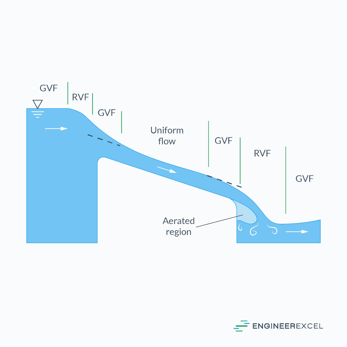
For example, backwater produced by a dam across a river and drawdown produced at a sudden drop in a channel can both be considered gradually varied flows, as illustrated in the diagram below.
In gradually varied flow, the bed slope, water surface slope, and energy slope will all have different values, and the flow velocity will vary along the channel. However, the basic assumption is that the bottom slope, water depth, and cross-section are all changing slowly. Additionally, the velocity distribution is one-dimensional, and the pressure distribution is approximately hydrostatic.
Therefore, unlike rapidly varied flow, gradually varied flow makes one-dimensional approximation valid and satisfies the continuity relation:
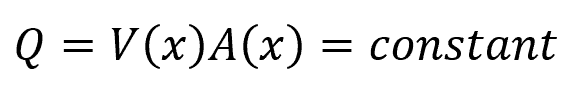
Where:
- Q = flow rate [m3/s]
- V = flow velocity [m/s]
- A = cross-sectional area of the flow [m2]
- x = longitudinal position along the flow channel [m]
Gradually Varied Flow Equation
A gradually varied flow can be characterized using the following equation:
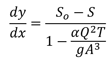
Where:
- y = depth of flow [m]
- So = slope of the channel bottom [unitless]
- S = slope of the energy grade line [unitless]
- α = kinetic energy correction factor [unitless]
- T = width of the channel [m]
- g = gravitational acceleration [9.81 m/s2]
This equation can also be expressed in terms of the Froude number as follows:
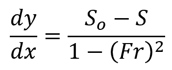
- Fr = Froude number [unitless]
The denominator can change sign, depending if the value of the Froude number is less than one (subcritical) or greater than one (supercritical). The numerator, on the other hand, can change sign depending if the slope of the channel bottom is greater than or less than the slope of the energy grade line.
The slope of the energy grade line is equivalent to the slope of a uniform flow at the same discharge Q. Hence, it can be calculated using the Chezy equation or the Manning equation as follows:
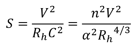
Where:
- Rh = hydraulic radius [m]
- C = Chezy coefficient [unitless]
- n = Manning roughness coefficient [unitless]
The value of the dimensionless parameter (α2) is 1.0 for SI units and 2.208 for BG units.
In addition to these equations, numerical solutions or approximate methods can be used to estimate gradual flow changes. Approximate methods are particularly valuable for natural channels with irregular cross sections and sparse, unevenly spaced data.
Channel Slope Classifications
Gradually varied flow can be categorized into five channel slope classifications based on the comparison between the actual channel slope (So) and the critical slope (Sc) or the slope of the critical depth. These classifications are steep slope, critical slope, mild slope, horizontal slope, and adverse slope.
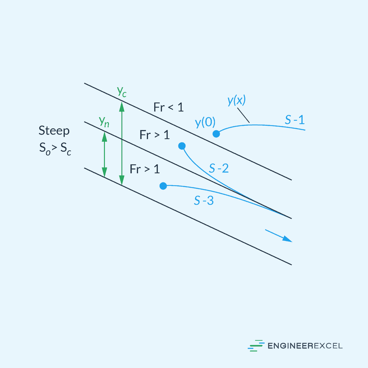
Steep Slope
A steep slope is characterized by a channel slope S₀ that is greater than the critical slope Sc for the same flow rate Q. In this case, the actual slope of the channel is steeper than the slope required for critical flow.
This results in a rapid flow that favors sediment transport and erosion. Example includes mountain streams, where water flows quickly due to steep slopes with possible presence of rocks or boulders.
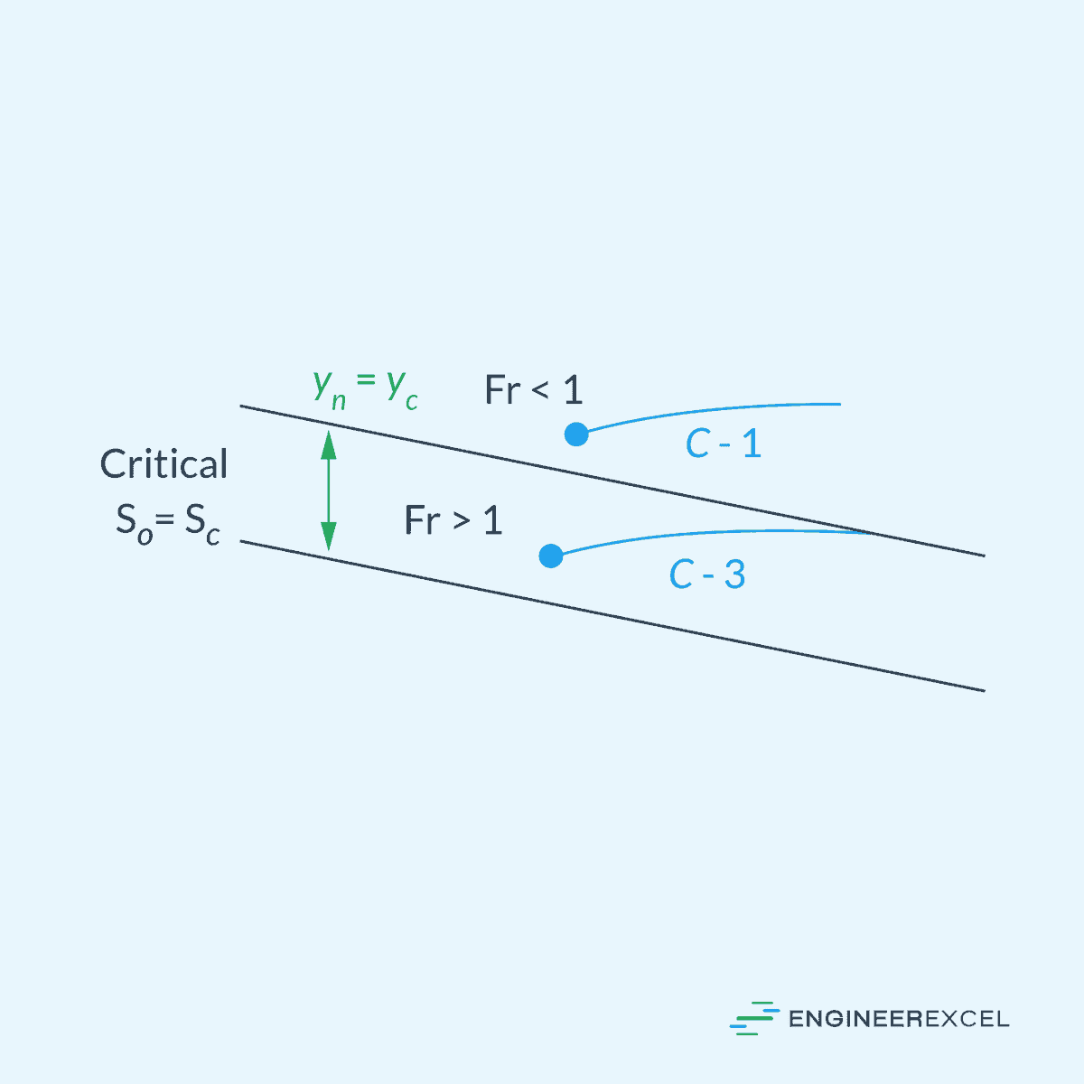
Critical Slope
In a critical slope, the channel slope S₀ is equal to the critical slope Sc. As a result, the normal flow is at its critical depth, forming a balance between gravitational and inertial forces. This state is typically unstable and can easily transition to either subcritical or supercritical flow if any changes occur.
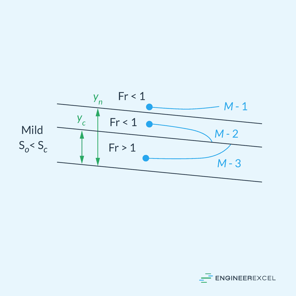
Mild Slope
Under a mild slope condition, the channel slope S₀ is less than the critical slope Sc. At a mild slope, the flow is subcritical and typically slower, resulting in sediment deposition. Example is a meandering river, where sediment deposit forms feature such as sandbars and riverbanks due to the slower flow rate.
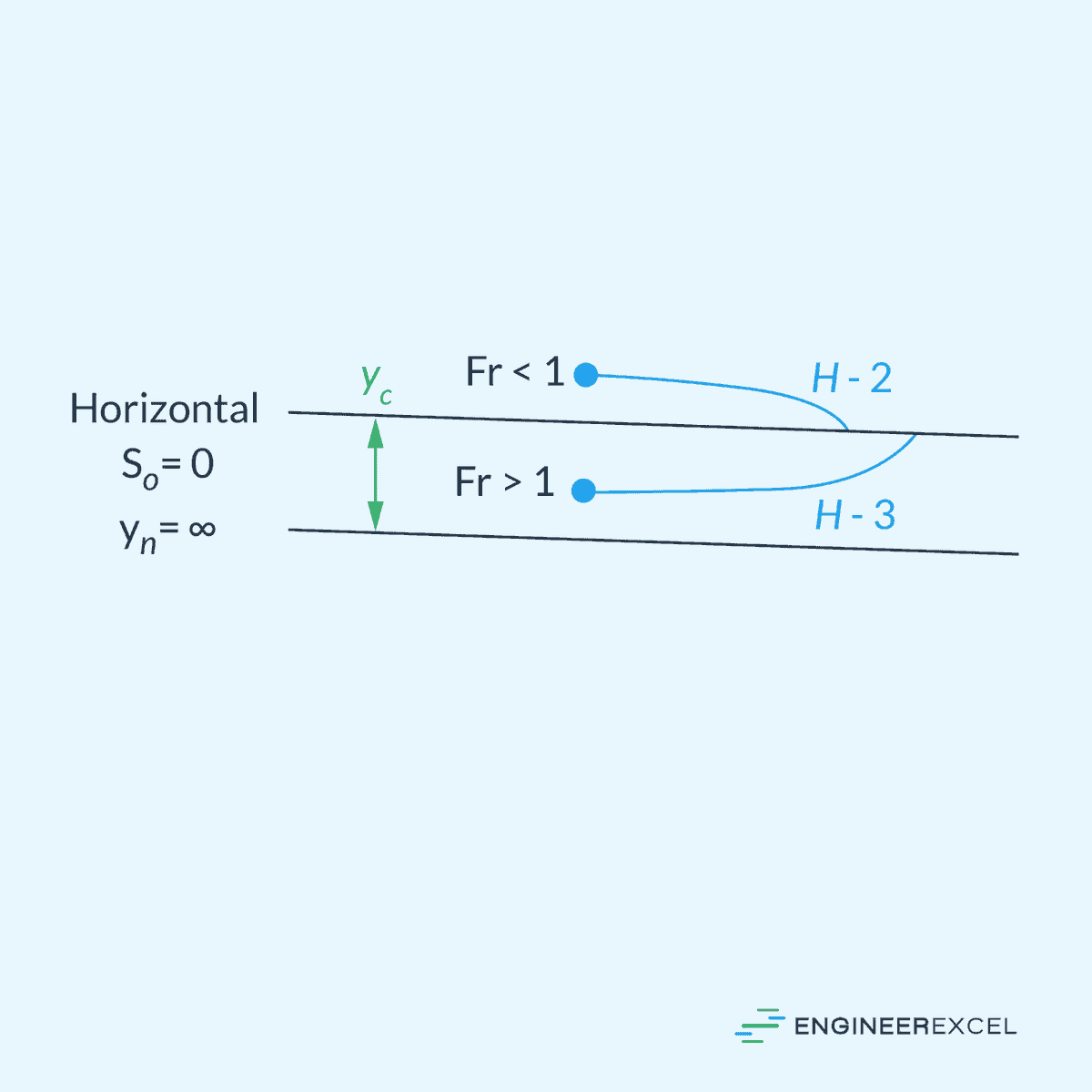
Horizontal Slope
Channels with a horizontal slope have no incline, and the channel slope S₀ is equal to zero. Horizontal slope channels often result in extremely slow subcritical flows, enabling sediment deposition and causing a potential increase in the water surface level. Example includes artificial drainage channels or canals, used in agricultural or urban settings to provide constant water supply with minimal gradient.
Adverse Slope
Lastly, an adverse slope refers to cases where the channel slope S₀ is negative, which means that the channel is inclined against the direction of the flow. Adverse slopes can cause water to pool and create backwater conditions, potentially leading to flooding. Example includes tidal estuaries, where shifts in tide may disrupt the natural flow by causing water to back up and create adverse slopes at the channel.
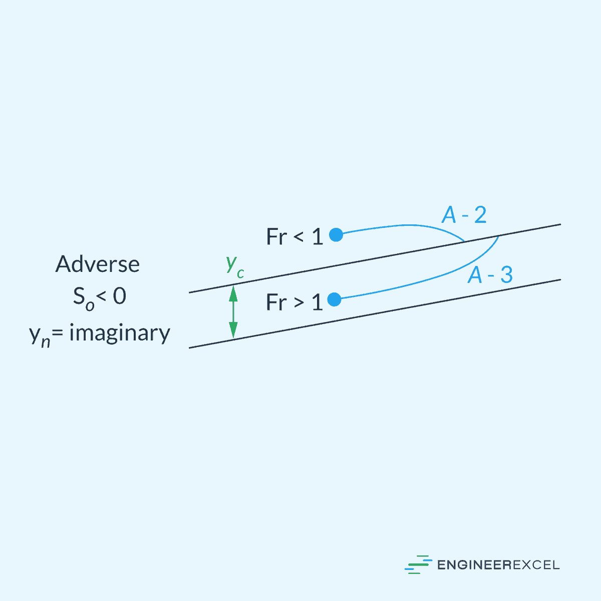
Collectively, these five categories result to twelve possible solution curves: three for steep slope (S-1, S-2, S-3), two for critical slope (C-1, C-3), three for mild slope (M-1, M-2, M-3), two for horizontal slope (H-2, H-3), and two for adverse slope (A-2, A-3). The letters S, C, M, H, and A represent the five types of slopes, while the numbers 1, 2, and 3 indicate the initial point’s position on the solution curve in relation to the normal depth yn and the critical depth yc.
In Type 1, the initial point is above both yn and yc, and in all instances, the water becomes even deeper than yn and yc as it moves along the channel. For Type 2 solutions, the initial point lies between yn and yc, and the water depth gradually approaches the lower of yn or yc asymptotically. In Type 3 cases, the initial point is below both yn and yc, and the solution curve gradually approaches the lower of yn or yc.