
In this post, you’ll learn how to perform constrained optimization in Excel through an example where we will maximize the flow rate in an open channel. The example will show that there is an optimal relationship between the channel dimensions that maximizes the flow rate for any required cross-sectional area.
If you aren’t interested in the problem setup, click here to go directly to the constrained optimization setup.
Video
Subscribe to EngineerExcel on YouTube
Constrained Optimization in Excel – Maximize Flow in an Open Channel
This example will demonstrate constrained optimization in Excel by maximizing the flow rate in an open channel with a trapezoidal cross-section.
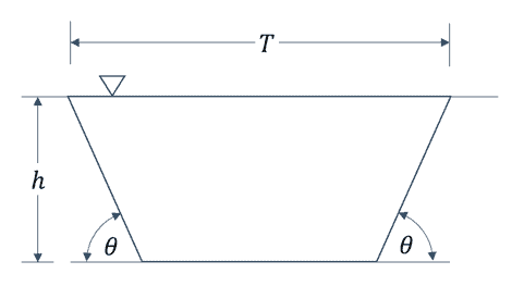
The geometry of the open channel is defined by three variables:

Elevate Your Engineering With Excel
Advance in Excel with engineering-focused training that equips you with the skills to streamline projects and accelerate your career.
- T, the top width
- h, the height
- θ, the angle of the side walls
Without any constraint on the cross-sectional area, the flow could be increased indefinitely by increasing any of the geometry variables.
However, if we place a constraint on the cross-sectional area, we will be able to find the optimum relationship between the three variables that provides for maximum flow
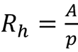
Flow in an open channel is maximized when the hydraulic radius of the geometry is greatest. So instead of maximizing the flow rate, which depends on other variables such as the slope of the channel of the channel, we can optimize the flow rate by maximizing the hydraulic radius. Hydraulic radius is defined as the cross-sectional area divided by the wetted perimeter:
Inputs
There are four inputs for this calculation:
- Top Width
- Height of the channel (depth of the water)
- Angle of the walls
- Target cross-sectional area
Placeholders are added for the time being and will be used as variables in the optimization we will set up in a later step. As always, units are added for clarity.
Outputs
There are four outputs which will be calculated:
- Bottom width of the trapezoidal channel (optional, but it makes subsequent calculations easier)
- Cross-sectional area
- Wetted perimeter
- Hydraulic radius
Constrained Optimization Steps
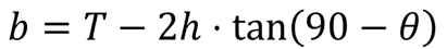
Step 1: Calculate the width at the bottom of the channel
The bottom width of the trapezoidal channel is calculated as a function of the top width, height, and side wall angle using the following equation:
The formula in Excel looks like this:
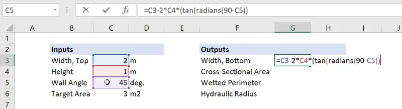
Remember that all trigonometric functions in Excel require the angle arguments to be in radians, so we use the RADIANS function to convert the angle from degrees before evaluating its tangent.
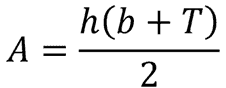
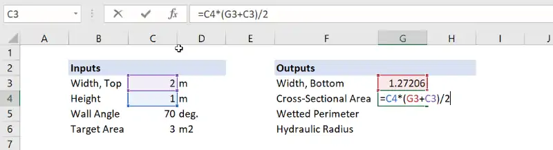
Step 2: Calculate the cross-sectional area in Excel
The cross-sectional area calculation for a trapezoid (where “b” is the bottom width) is straightforward:
And here is the formula in Excel:
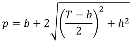
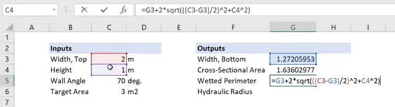
Step 3: Calculate the wetted perimeter
The calculation for wetted perimeter is probably the most difficult one in this spreadsheet:
This is the formula in Excel:
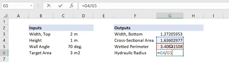
Step 4: Calculate the hydraulic radius
The hydraulic radius is the final output to be calculated in the spreadsheet. It is simple the area divided by the wetted perimeter, and we end up with a value of about 0.48 meters.
Step 5: Open Solver and set the objective
We can use the Solver add-in to run this constrained optimization in Excel. The Solver add-in is opened through a button on the far-right side of the Data tab. (If you don’t see it, that probably means you need to enable the Solver add-in.)
Once open, we need to tell Solver which cell result we want to optimize. This is known as the Objective Cell. In our example, we will be maximizing the hydraulic radius, which is the results in cell G6.
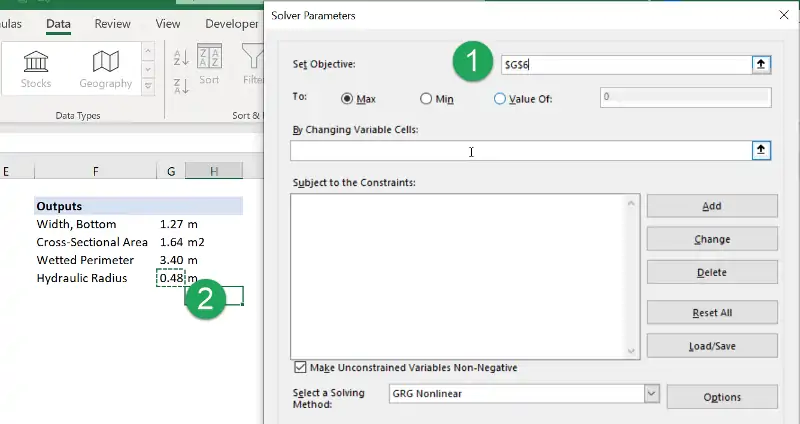
The default behavior in Solver is to maximize the result.
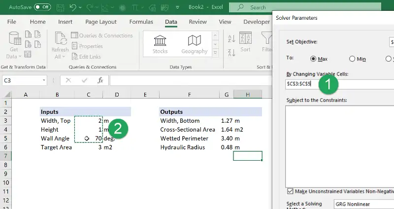
Step 6: Set the Solver variables
Once the objective has been defined, Solver will also need information on which cells to modify to achieve the objective. In the diagram at the beginning of this post, we identified those variables as the top width, the height, and the wall angle.
Click in the field “By Changing Variable Cells:” and select cells C3:C5.
Step 7: Set up the constrained optimization in Excel Solver
Without a constraint on this problem, Solver would target an infinite hydraulic radius by increasing the top width and height to infinity (for any wall angle).
To prevent this behavior, a constraint is added which will force Solver to stay within some limits. This is referred to as constrained optimization.
A constraint can be placed on an objective cell, variable cell, or any cell in the worksheet.
To constrain this optimization problem, first click on the “Add” button on the right side of the Solver window to open the “Add Constraint” window:
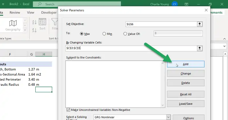
After the new window opens, the constrained cell is set as follows:
- Click in the “Cell Reference” field
- Select the cell value to be constrained
- Click in the “Constraint” field
- Choose the cell containing the constraint value
In our case, the “cell reference” is the value of the cross-sectional area and the “constraint” is the value of the target area. The constraint could also be a numerical value, but it’s a best practice to choose a cell.
Finally, set the constraint behavior in the middle field. Either “≤” or “=” are valid selections in this case.
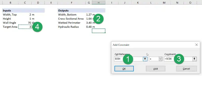
Once all the fields are set, click “OK” and the constraint will be added to Solver.
Results
After clicking the “Solve” button in Solver, the constrained optimization will be completed in just a few seconds and we can examine the results.
The first thing to notice is that the constraint has been obeyed because the output cross-sectional area is equal to the target area.
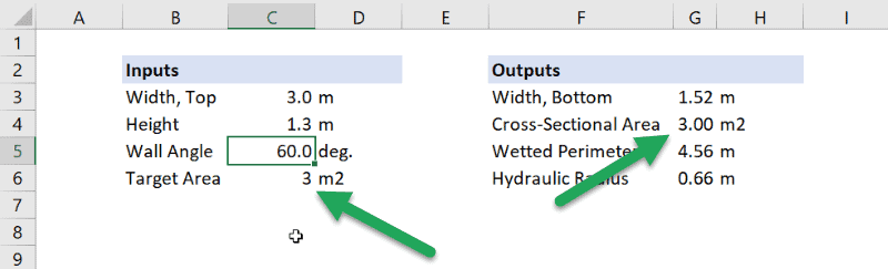
Additionally, Solver has optimized the values of the top width, height, and wall angle to some values.
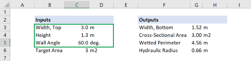
The thing that stands out most about this is that the optimal wall angle is 60 degrees, which is the same as the angle between the sides of a hexagon. This seems reasonable, because we would expect the wetted perimeter to decrease (and hydraulic radius to increase) as the geometry of the open channel becomes more like a semicircle. Also, the ratio between the top width and height is equal to 2.3. Let’s see if these relationships hold up for a different cross-sectional area target.
Change the target area to 5 m^2 and rerun the optimization in Solver to get the following results:
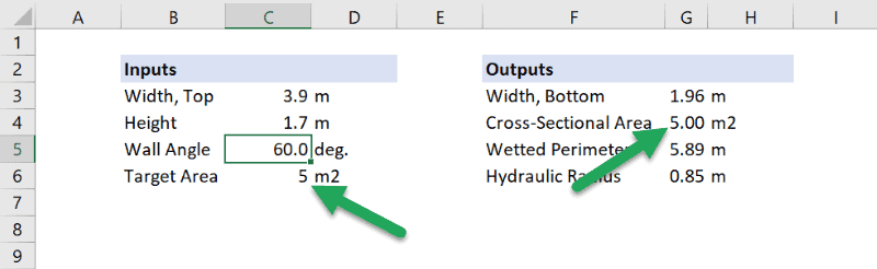
Once again, the constraint has been obeyed, the wall angle is 60 degrees, and the ratio of the top width to height is 2.3. It looks like we’ve found an optimal geometry relationship for flow through an open channel!