
Complex piping systems that include branched pipe flow are commonly encountered in various industries, particularly those that rely heavily on piping distribution networks, such as water distribution systems, oil and gas transport, and process industries.

In this article, we will delve into the fundamentals of branched pipe flow calculations and their significance in engineering applications.
Branched Pipe Flow Calculations
Branched pipe systems involve pipes of different diameters, materials, and lengths connected at nodes, where flow is divided or combined. They are common in various engineering applications, including water supply, oil and gas distribution, and HVAC systems.
Analyzing branched pipe systems requires consideration of the same factors as single pipe systems, such as fluid properties, pipe characteristics, and flow rates. They are also governed by the same principles such as the conservation of mass and energy principles, as well as the calculation of head losses due to pipe friction and minor losses in fittings and valves. The difference lies in complexity.

Elevate Your Engineering With Excel
Advance in Excel with engineering-focused training that equips you with the skills to streamline projects and accelerate your career.
Due to complexity, calculation of flow rates and pressure drops in branched pipe systems often need simultaneous manipulation of multiple equations and involve more variables. In this article, the discussion will be divided into three types of branched pipe systems: pipes in parallel, three-reservoir junction, and piping networks.
Pipes in Parallel
Pipes in parallel are pipes that are connected so that the flow from a pipe branches or divides into two or more separate pipes and then reunites into a single pipe, as shown in the diagram below.
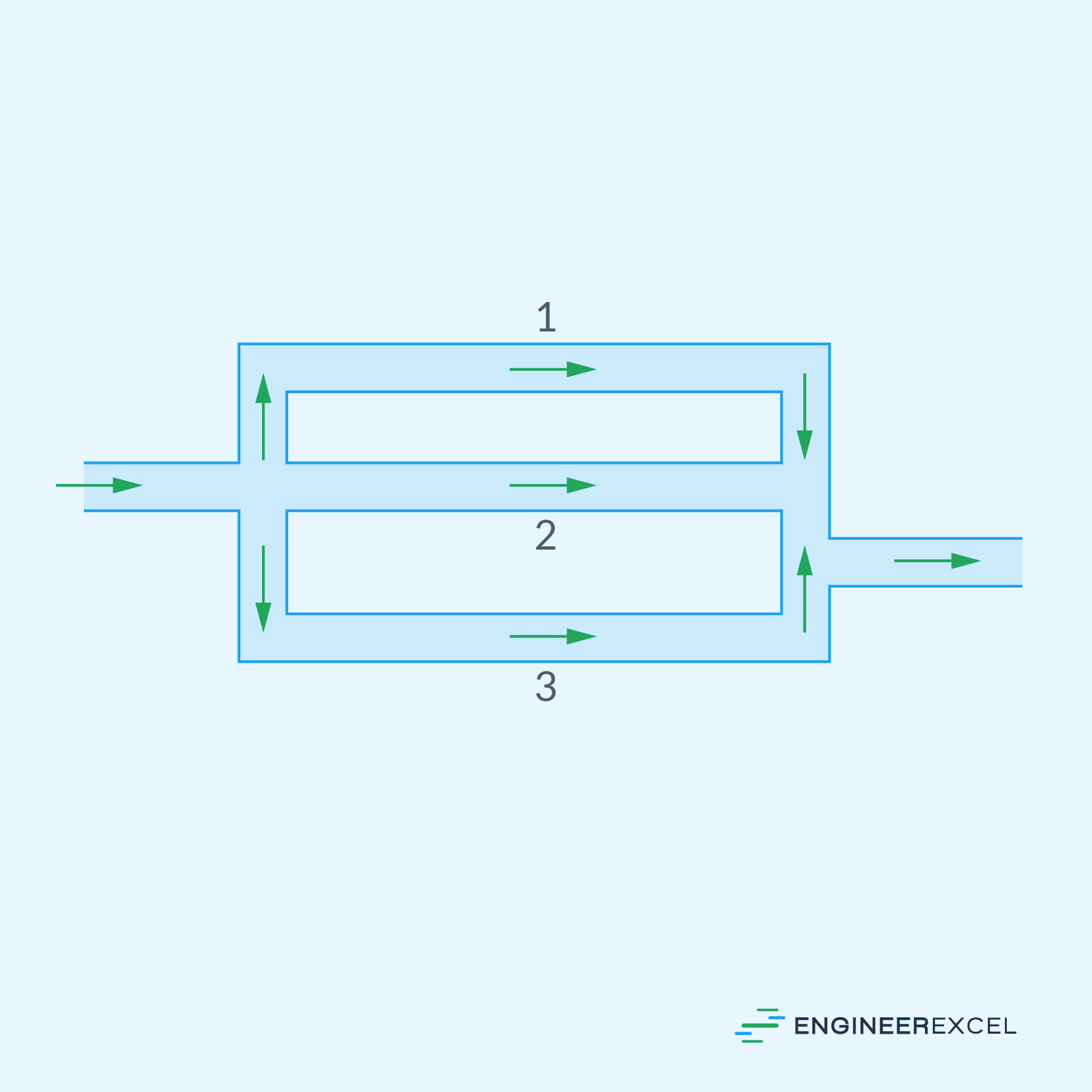
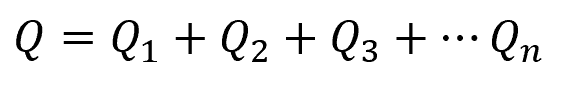
In this arrangement, the total flow rate divides among the branch pipes, such that:
Where:
- Q = total flow rate [m3/s]
- Qn = flow rate in each individual branch [m3/s]
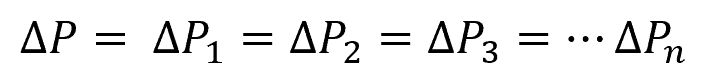
In addition, the pressure drop is assumed to be the same in each pipe, such that:
Where:
- ΔP = total pressure drop [Pa]
- ΔPn = pressure drop across each branch [Pa]
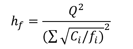
In this configuration, the total head loss can be related to the total flow rate using the following equation:
Where:
- hf = total head loss [m]
- fi = friction factor for each pipe branch [unitless]
In the above formula, the value of Ci for each branch can be calculated using the following equation:
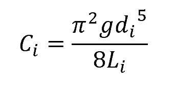
Where:
- di = internal diameter of each pipe branch [m]
- Li = length of each pipe branch [m]
- g = gravitational acceleration [9.81 m/s2]
It is important to note that the value of the friction factor varies with roughness ratio and Reynolds number which, in turn, varies with flow rate. Hence, it is necessary to solve the above equations using iterative methods.
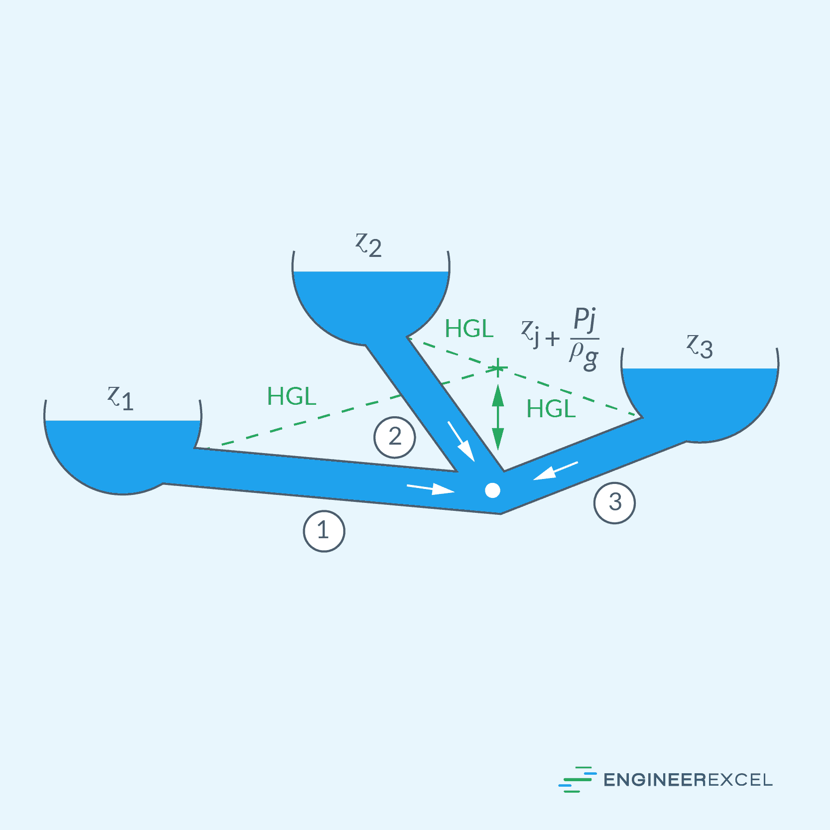
Three-Reservoir Junction
A three-reservoir junction is a system where three reservoirs are connected by pipes at a common junction, as shown in the diagram below.
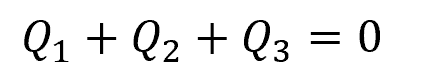
In a three-reservoir pipe junction, the flow rates are considered to cancel out at the junction such that:
Assuming that the gauge pressure at each of the reservoir surface is zero, the head loss through each branch can be calculated using the following set of equations:
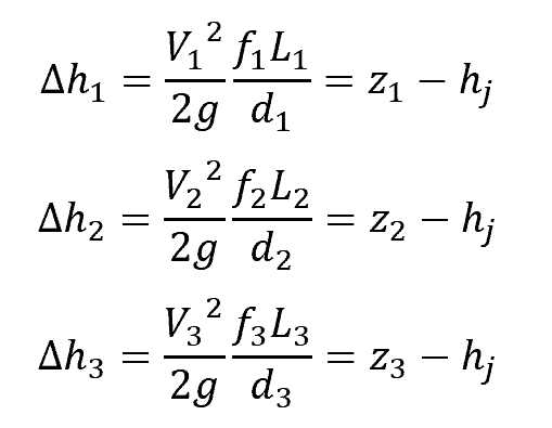
Where:
- Δhi = head loss through each branch [m]
- Vi = fluid velocity through each branch [m]
- zi = elevation of each reservoir [m]
- hj = elevation of the hydraulic grade line at the junction [m]
In the above equations, the elevation of the hydraulic grade line at the junction is given by the formula:
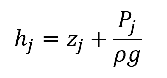
Where:
- zj = elevation at the junction [m]
- Pj = static pressure at the junction [m]
- ρ = fluid density [kg/m3]
Using iterative method, the above set of equations can be used to calculate for the flow velocity at each branch, which can then be used to calculate for the flow rates. The iteration is done until the flow rates balance at the junction.
Piping Networks
The ultimate case of a branched pipe system is a piping network, which is illustrated in the diagram below.
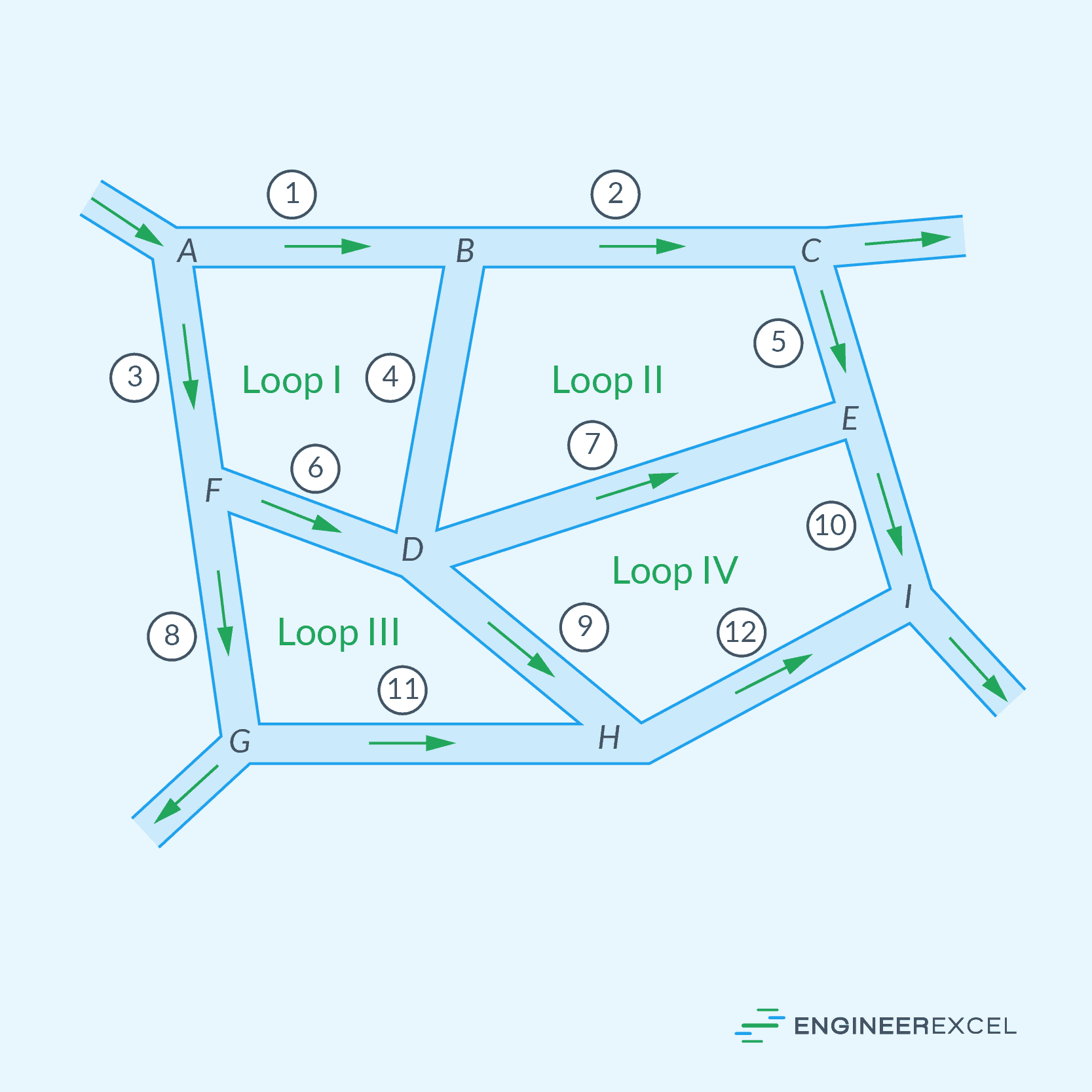
Although this is much bigger and more complex than the previously discussed configurations, it generally follows the same basic rules:
- The net flow into any junction is zero.
- The pressure difference around any closed loop is zero.
- All pressure losses satisfy the major and minor loss friction correlations.
Using these rules, a set of equations for each junction and independent loop in the piping network can be set up, which can then be solved simultaneously using numerical iteration.
Two of the most popular methods used to analyze piping networks are Hardy Cross and Newton-Raphson. Hardy Cross is a popular iterative technique that balances the head losses around closed loops within the branched system. Each iteration adjusts the flow rates until the summed head losses around the loops are negligible.
Newton-Raphson, on the other hand, is an iterative method that uses partial derivatives of the system equations to approximate a solution. This approach can provide improved convergence and faster results for complex systems.
Applications of Branched Pipe Systems
Branched pipe systems can be found in various applications. In water supply systems, for example, branched pipe networks are crucial for distributing water to different areas of a community or industry. You may encounter pipes branching off from larger mains to deliver water to smaller networks, like neighborhoods or individual buildings.
In oil and gas industries, the transportation of oil and gas from extraction sites to refineries and distribution centers often relies on intricate pipeline networks. These industries often require a more careful consideration of properties such as fluid viscosity, temperature, and changes in elevation.
Lastly, Heating, Ventilation, and Air Conditioning (HVAC) systems also utilize branched pipe networks to distribute conditioned air or heating and cooling fluids throughout a building. In these systems, proper sizing of ducts and pipes, as well as balancing the airflow or fluid flow among the different branches, is crucial for maintaining comfort and efficiency.