


3 Axis Graph Excel Method: Add a Third Y-Axis
Ever wanted to know how to create a 3 axis graph in Excel? The other day I got a question from Todd, an EngineerExcel.com subscriber.

Linear Interpolation in Excel
To perform linear interpolation in Excel, use the FORECAST function to interpolate between two pairs of x- and y-values directly. In the example below, the

Curve Fitting in Excel
I’ve discussed linear regression on this blog before, but quite often a straight line is not the best way to represent your data. For these
Anisotropic Materials: Directionally Dependent Material Behavior
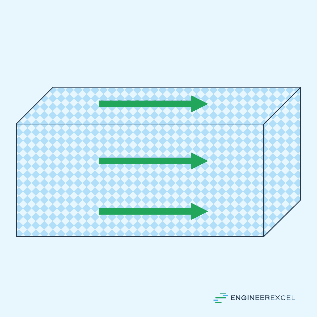
Anisotropic materials are substances whose properties vary depending on the direction in which they are measured or observed. Unlike isotropic materials, which exhibit uniform properties
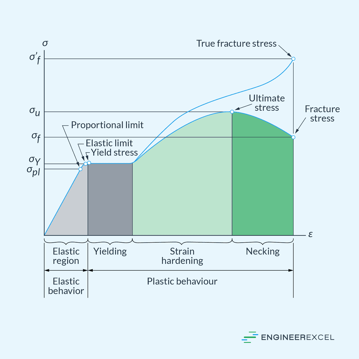
Modulus of Elasticity: Quantifying Stiffness of Materials
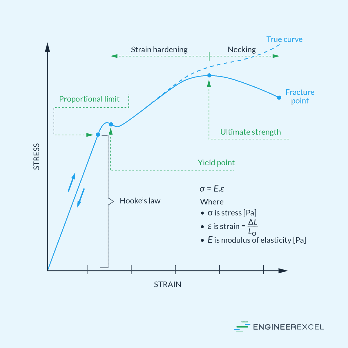
Modulus of elasticity is a measure of a material’s stiffness or resistance to deformation when subjected to stress. It quantifies how much a material will
Understanding Axial Deformation in Engineering Materials
Axial deformation refers to the change in length of a material along its longitudinal axis under applied force or load. It typically occurs in structures