To perform linear interpolation in Excel,  use the FORECAST function to interpolate between two pairs of x- and y-values directly.

In the example below, the formula to interpolate and find the y-value that corresponds to an x-value of 1.4 is:

=FORECAST(F2,C3:C4,B3:B4)

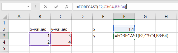
This simple method works when there are only two pairs of x- and y-values. If there are more than 2 pairs, the calculation is more complex.

Linear Interpolation in Excel

There isn’t a linear interpolation function in Excel , but the FORECAST function can be used for linear interpolation when there are just two pairs of x- and y-values.

It has the following syntax:

=FORECAST(x,known_ys,known_xs)

where:

• x is the input value
• known_ys are the known y-values
• known_xs are the known x-values

The FORECAST function works by using linear regression to estimate the value of y that corresponds to the input value x. When there are only two data points, the result of linear regression is the same as linear interpolation.

However, when the number of x-values and y-values is greater than 2, the result of the FORECAST function will NOT be an interpolated y-value.

To interpolate between x- and y-values in a large data set (more than 2 pairs of values), use either XLOOKUP or INDEX and MATCH to extract a pair of x- and y-values to interpolate between.

Linear interpolation assumes that the change in y for a given change in x is linear. In most cases linear interpolation in Excel will provide results that are sufficiently accurate. However, if you need even greater accuracy, you may want to consider a more advanced method such as cubic splines.

Interpolate in Excel with XLOOKUP

If you are a Microsoft 365 subscriber, or are using Excel 2021, Excel for the web, or Excel for iOS or Android devices, you can use the XLOOKUP function to extract the values. If you are on an older version of Excel, use the INDEX/MATCH method described below.

In some other posts on looking up tabular data in Excel, I’ve focused on how to extract known x- and y-values from a table. But what if you need to interpolate missing data in Excel for better accuracy? Well, it’s also possible to perform linear interpolation in Excel, which enables you to estimate a y-value for any x-value that is not provided explicitly in the data.

Let’s look at how to interpolate in Excel on some real data.

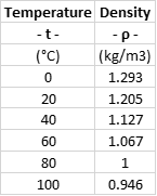
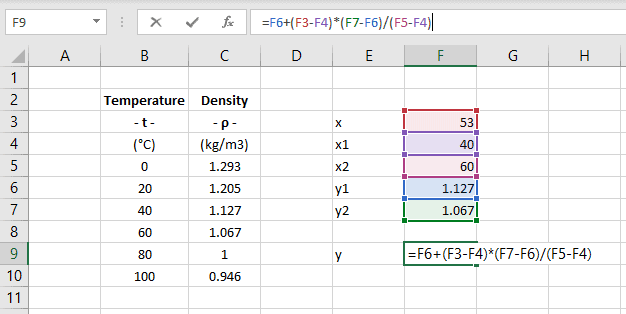
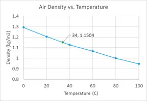
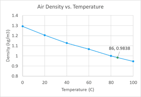
The table below lists air density as a function of temperature in 20-degree Celsius increments. To get data at any temperature between 0 and 100 C, we’ll have to interpolate.

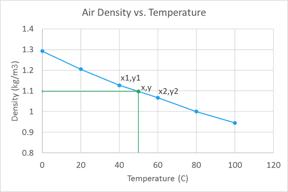
To estimate the density at 53 degrees Celsius, use XLOOKUP to find the values x1=40, y1=1.127, x2=60, and y2=1.067 in the table, then feed those values into the FORECAST function to perform the interpolation.

Use XLOOKUP to Find Values to Interpolate in Excel

XLOOKUP has the following syntax:

=XLOOKUP(lookup_value, lookup_array, return_array, [if_not_found], [match_mode], [search_mode])

where

• lookup_value is the value to find
• lookup_array is the array where the lookup_value is searched for
• return_array is the array from which a result is returned
• if_not_found is the value to return if nothing is found (optional)
• match_mode tells the function what to do if an exact match is not found (optional)
• search_mode tells the function how to search the array (optional)

To interpolate in Excel, use the XLOOKUP function to find the x-values on either side of the input value of x as well as the corresponding y-values.

To find the first x-value from the table of data, use the following formula:

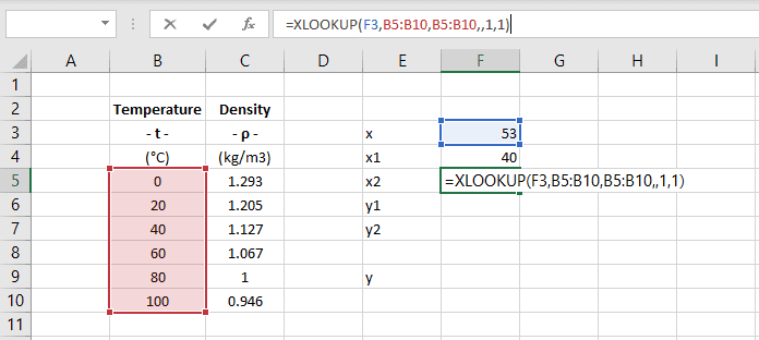
=XLOOKUP(F3,B5:B10,B5:B10,,-1,1)

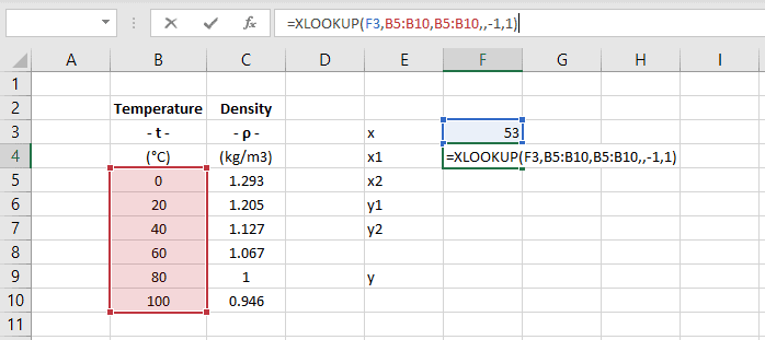
F3 is the lookup_value, and the array B5:B10 is both the lookup_array and the return_array. Setting the match_mode to -1 tells the function to return the next smaller item in the return array and setting the search_mode to 1 starts the search from the top of the array.

The resulting value of x1 is 40, which is the greatest temperature that is less than 53, the x-value.

A very similar formula is used to find the value of x2:

=XLOOKUP(F3,B5:B10,B5:B10,,1,1)

The only difference is that match_mode is set to 1 (rather than -1), because x2 is the next largest value in the return array.

The resulting value of x2 is 60, the lowest temperature greater than 53 in the lookup array.

Next, find the corresponding y-values y1 and y2 using XLOOKUP. For y1, F3 is the lookup_value and B5:B10 is the lookup_array, just as before. To return a y-value that corresponds to an x-value less than the lookup_value, C5:C10 is the return_array and the match_mode is -1.

=XLOOKUP(F3,B5:B10,C5:C10,,-1,1)

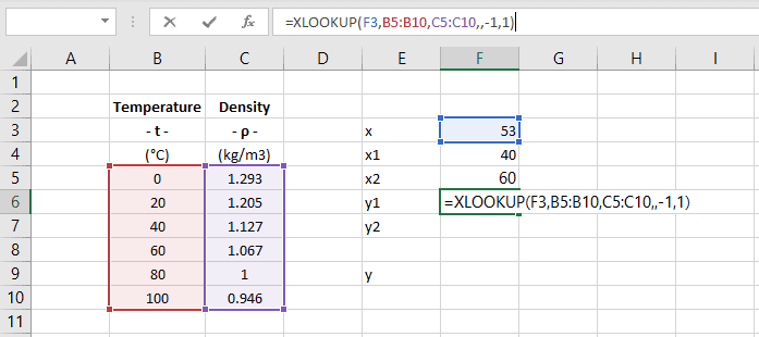
y1 is equal to 1.127.

The last value to lookup is y2. The formula is just slightly different from the formula for y1. match_mode is set to 1 to return the next largest value of y:

=XLOOKUP(F3,B5:B10,C5:C10,,1,1)

Use FORECAST for Excel Interpolation

Once 2 pairs of x- and y-values are known, FORECAST can be used to interpolate between them to estimate the y-value for a given x-value with the following formula:

=FORECAST(F3,F6:F7,F4:F5)

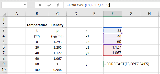
The estimate for y is 1.088.

Prevent Excel Interpolation Errors

An error can occur when the value of x is equal to one of the x-values in the lookup array. This causes x1 to be equal to x2 and y1 to be equal to y2. When this happens, FORECAST cannot calculate a slope and returns an error.

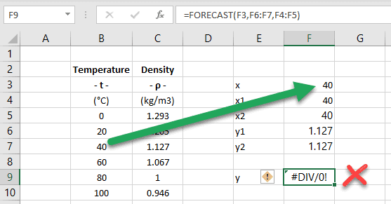
The error can be prevented by wrapping the FORECAST function in an IF function that checks if the values of x and x1 are equal.

If x and x1 are equal, y is equal to y1.

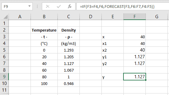
=IF(F3=F4,F6,FORECAST(F3,F6:F7,F4:F5))

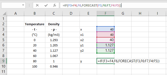
This formula correctly returns a result of 1.127 when x is equal to 40.

Use the INDEX/MATCH Functions for Interpolation in Excel

If you are not a Microsoft 365 subscriber or are using an older version of Excel, the XLOOKUP function is not included.

No worries though!

You can use the INDEX and MATCH functions to get the same results. The syntax for these functions is explained here, so if you need a refresher be sure to check that out.

RELATED: USING EXCEL’S INDEX AND MATCH FUNCTIONS TO LOOK UP ENGINEERING DATA

MATCH returns the location of a value (n) in a column or row of data.

INDEX returns the actual value in the n^th position of a row or column of data.

By using these functions together, we can extract the values of x1, y1, x2, and y2 we need for the interpolation.

Find the value of x1 with this formula:

=INDEX(B5:B10,MATCH(F3,B5:B10,1))

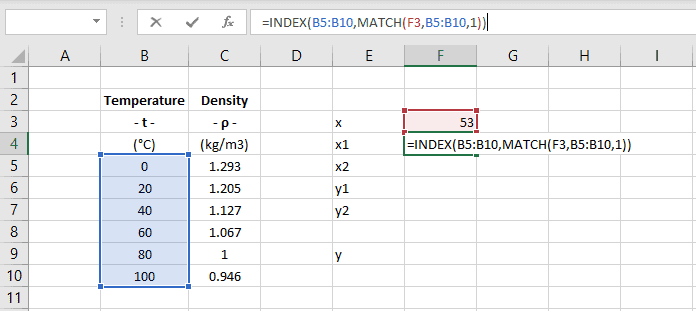
The formula returns 40 because the match_type argument in the MATCH function is set to 1. This tells the MATCH function to return a position from the temperature array that is less than the lookup_value when an exact match is not found.

Find the value of x2 with this formula:

=INDEX(B5:B10,MATCH(F3,B5:B10,1)+1)

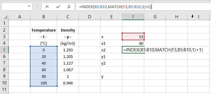
The formula for x2 returns 60 because the result returned by the MATCH function is increased by 1 to tell Excel to lookup the next row in the array.

For y1 and y2 the formulas are very similar. The only difference is that the array argument for the INDEX function is column C.

For y1, the formula is:

=INDEX(C5:C10,MATCH(F3,B5:B10,1))

For y2, the formula is:

=INDEX(C5:C10,MATCH(F3,B5:B10,1)+1)

Finally, use the FORECAST function as described above to return the estimated value of y:

=FORECAST(F3,F6:F7,F4:F5)

How to Interpolate in Excel with the Interpolation Formula

It’s also possible perform linear interpolation in Excel without using the FORECAST function. Instead, use the interpolation formula below, where y is the value to return, and x is the independent variable:

This formula can be used in Excel to linearly interpolate the value of y:

=F6+(F3-F4)*(F7-F6)/(F5-F4)

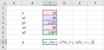
[Hint] Use Named Cells to make the formula much easier to understand:

How do you interpolate a graph in Excel?

The interpolation results can be shown on a graph by creating an Excel chart with two data series. The first series consists of the arrays of x- and y-values. The second series contains the x value to look up and the resulting estimate of y.

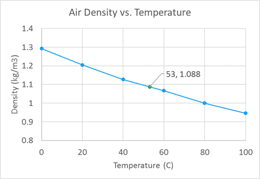
The great thing about setting the formulas up as demonstrated above is that you can interpolate correctly between ANY pair of known x- and y- values.

Wrap-Up

So there you are – several alternate methods to perform linear interpolation in Excel. Hopefully you can use one of these methods to save time when you need to interpolate data from a large data set.