
I’ve discussed on this blog before, but quite often a straight line is not the best way to represent your . For these specific situations, we can take advantage of some of the tools available to perform or in .
in with Charts
charts are a convenient way to fit a to .
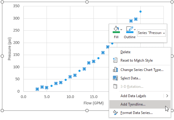
First, create a scatter .
Then right click on the series and select “Add …”

Elevate Your Engineering With Excel
Advance in Excel with engineering-focused training that equips you with the skills to streamline projects and accelerate your career.
In the Format pane, select the options to on and Display R-Squared on .
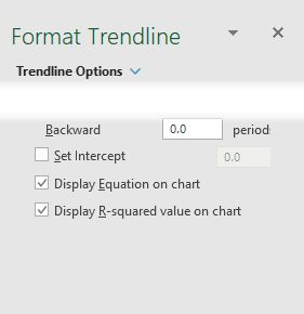
Try different types of curves to see which one maximizes the of R-squared.
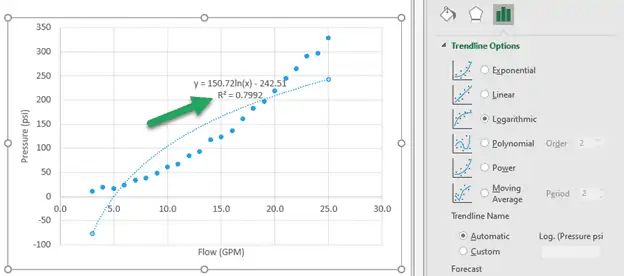
For this set, a logarithmic fits the with an R-squared of 0.7992. From the image below, we can also clearly see that it is not a good fit.
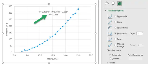
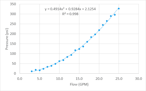
However, a second-order polynomial fits the with an R-squared of 0.998. That means the fits the better.
Although the option is convenient, it may not always be the best option when you want to know the that best fits the .
In some cases, it may provide only 1 or 2 significant digits for the . This will make any formula that uses these only accurate to the same number of significant digits.
Also, there is no way to reference the of the in the spreadsheet without manually typing them into cells. This can cause problems if the is updated, and the are not updated in the spreadsheets.
However, there is an option that provides a robust way to in using the .
in
Remember our old friend LINEST? Although LINEST is short for “linear estimation”, we can also use it for nonlinear with a few simple tweaks.
LINEST has the following syntax:
= LINEST(known_y’s, [known_x’s], [const], [stats])
where
- known_y’s are the y-values corresponding to the x-values which you are trying to fit (or )
- known_x’s are the known x-values (or )
- const (optional) is set to TRUE for the y-intercept to be calculated normally and set to FALSE if the y-intercept should be set to ZERO
- stats (optional) is an argument that tells whether to return . TRUE will return the statistics and FALSE will return no statistics.
Polynomial in
Let’s say we have some of pressure drop vs. flow rate through a water valve, and after plotting the on a we see that the is quadratic, as in the example above.
Even though this is nonlinear, the can also be used here to find the best fit for this . For a , we do that by using array constants .
An advantage to using LINEST to get the that define the is that we can return the directly to cells. That way we don’t have to manually transfer them out of the .
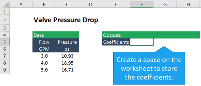
Since the is quadratic, or a second order polynomial, there are three , one for x squared, one for x, and a constant. So we’ll need to start by creating a space to store the three for the .
Using LINEST for in
The returns an array of , and optional . So we’ll need to enter it as an array formula by selecting all three of the cells for the before entering the formula.
If the cells containing the flow and pressure are named “flow” and “pressure”, the formula looks like this:
=LINEST(pressure, flow^{1,2},TRUE, FALSE)
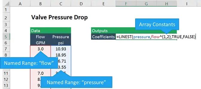
The known y’s in this case are the pressure measurements, and the known x’s are the flow measurements raised to the first and second power. The curly brackets, “{” and “}”, indicate an array constant in . Basically, we are telling to create two arrays: one of flow and another of flow-squared, and to fit the pressure to both of those arrays together.
Finally, the TRUE and FALSE arguments tell the to calculate the y-intercept normally (rather than force it to zero) and not to return additional , respectively.
Since it’s an array formula, we need to enter it by typing Ctrl+Shift+Enter .
The then returns the of x 2 and x as well as a constant (because we chose to allow LINEST to calculate the y-intercept).
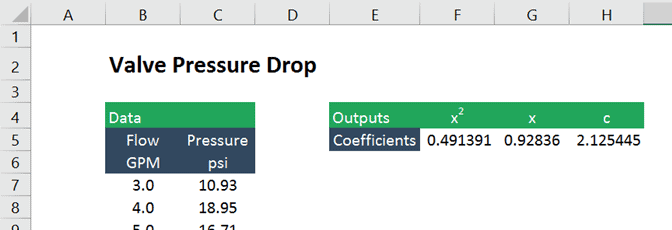
The are identical to those generated by the tool, but they are in cells now which makes them much easier to use in subsequent calculations.
For any , LINEST returns the coefficient for the highest order of the on the far left side, followed by the next highest and so on, and finally the constant.
A similar technique can be used for Exponential, Logarithmic, and Power in as well.
a Logarithmic to
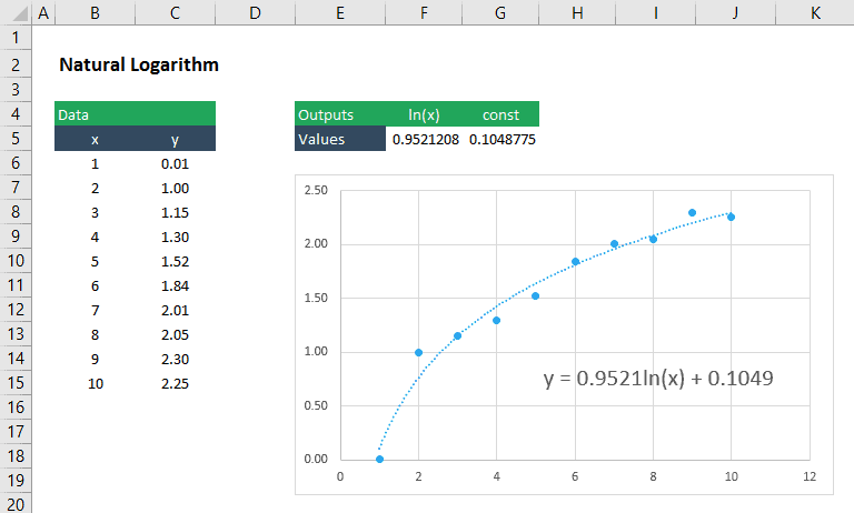
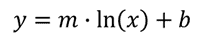
A logarithmic function has the form:
We can still use LINEST to find the coefficient, m , and constant, b , for this by inserting ln(x) as the argument for the known_x’s:
=LINEST(y_values,ln(x_values),TRUE,FALSE)
Of course, this method applies to any logarithmic , regardless of the base number. So it could be applied to an containing log10 or log2 just as easily.
in
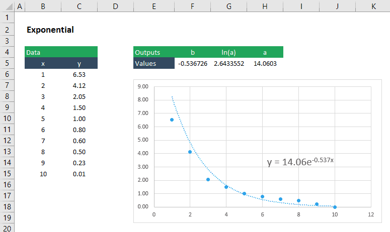
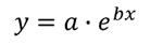
An exponential function has the form:
It’s a little trickier to get the a and b for this because first we need to do a little algebra to make the take on a “linear” form. First, take the natural log of both sides of the to get the following:
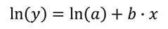
Now we can use LINEST to get ln(a) and b by entering ln(y) as the argument for the y_values:
=LINEST(ln(y_values),x_values,TRUE,FALSE)
The second returned by this array formula is ln(a), so to get just “a” , we would simply use the exponential :
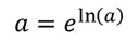
Which, in an , translates to:
=EXP(number)
a Power to
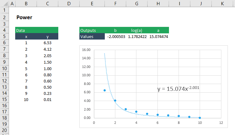
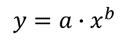
A power can be fit to using LINEST in much the same way that we do it for an exponential . A power has the form:
Again, we can “linearize” it by taking the base 10 log of both sides of the to obtain:
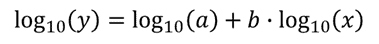
With the in this form, the to return b and log 10 (a) can be set up like this:
=LINEST(LOG10(yvalues),LOG10(xvalues),TRUE,FALSE)
Since the returns b and log10(a) , we’ll have to find a with the following formula:
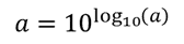
In , that formula is:
=10^(number)
That’s it for now. As you can see, there are a number of ways to use the for nonlinear in .