
Laminar flow refers to the smooth flow of fluids with little or no mixing between adjacent layers. In laminar flow, the fluid particles flow predictably in a well-ordered fashion, following a linear path without turbulent motion or chaotic swirling.

In this article, we will discuss the hydraulics of laminar flow, including its principles, equations, and applications.
Defining Laminar Flow
In laminar flow, the fluid moves in smooth, parallel layers or laminae, with each layer having a relatively constant velocity and direction. Because there is minimal random motion or eddying of the fluid particles, adjacent layers do not mix or disrupt each other. Hence, the flow is orderly and stable.
This makes the flow profile of laminar flow predictable. That is, the velocity of the fluid at any given point within the flow is well-defined and can be calculated or predicted using mathematical equations. Presently, with increases in computer speed and memory, almost any laminar flow can be modeled accurately.

Elevate Your Engineering With Excel
Advance in Excel with engineering-focused training that equips you with the skills to streamline projects and accelerate your career.
Laminar Flow Hydraulics
Reynolds Number for Laminar Flow
Reynolds number is a dimensionless quantity used in fluid mechanics to predict the flow regime by measuring the ratio between inertial and viscous forces. In reality, the transition between regimes depends on many factors, such as wall roughness or fluctuations in the inlet stream, but the
primary parameter is the Reynolds number.
Laminar flow typically occurs at low Reynolds numbers. The critical Reynolds number for the transition from laminar to turbulent flow can vary depending on the specific conditions and geometry of the flow.
The table below lists the critical Reynolds numbers for some of the most common geometries for laminar flow.
| Geometry | Critical Reynolds Number for laminar flow |
| Flow in pipe | 2300 |
| Flow along a flat plate | 500,000 |
| Flow across a sphere | 24 |
| Flow across a symmetric wedge | 200-2,000, depending on orientation angle |
| Flow across a cylinder | 30 |
Entrance Length of Laminar Flow
When a fluid flows into a pipe or duct from a reservoir or inlet, it undergoes changes in velocity and velocity profile as it progresses along the length of the conduit. In fluid dynamics, the entrance length is the distance over which the fluid flow develops from an initial, non-uniform state to a fully developed, uniform state.
For laminar flow, the accepted correlation for the entrance length is:
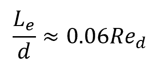
Where:
- Le = entrance length [m]
- d = diameter of the conduit [m]
- Red = Reynolds number [unitless]
Velocity Profile of Laminar Flow
Laminar flows generally have a well-defined fully-developed velocity profile. However, its specific shape depends on the geometry of the flow.
In circular pipe flow, for example, the fully-developed velocity profile tends to be parabolic. This can be expressed as a function of the radial distance from the center of the pipe as follows:
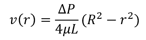
Where:
- v(r) = velocity of the fluid at a radial distance r from the center of the pipe [m/s]
- ΔP = pressure difference between the two ends of the pipe [Pa]
- μ = dynamic viscosity of the fluid [Pa-s]
- L = pipe length [m]
- R = pipe radius [m]
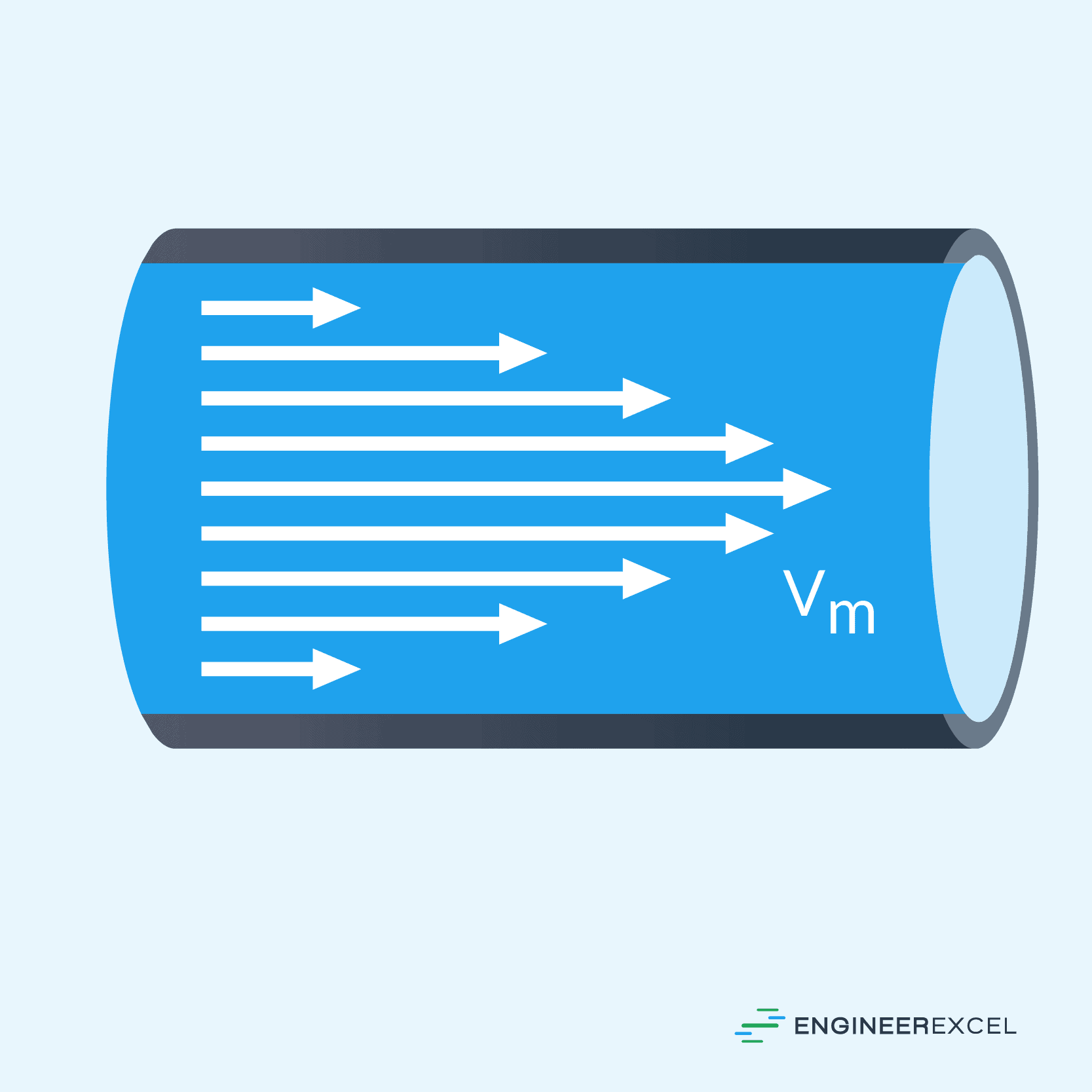
The typical velocity profile of a circular pipe flow is illustrated in the diagram below.
Nusselt Number for Laminar Flow
The Nusselt number is the ratio between the convective and conductive components of heat transfer across a boundary layer of fluid. In this context, convective heat transfer involves the transfer of heat due to both fluid movement and conduction, while conductive heat transfer only considers heat conduction in a fluid that is hypothetically stationary under the same conditions. The Nusselt number is normally used to obtain the value of the heat transfer coefficient.
For laminar flows, the Nusselt number typically falls within the range of 1 to 10. However, its exact value depends on several factors, including the flow’s location with respect to the entrance region and the specific boundary conditions of the system.
For a laminar pipe flow at constant wall temperature, the following empirical relation, developed by Hausen, can be used to calculate for the Nusselt number:
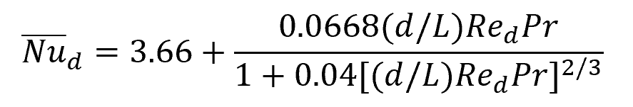
Where:
- Nud = average Nusselt number across the pipe length [unitless]
- Pr = Prandtl number [unitless]
For a thermally fully developed laminar pipe flow at constant heat flux, the Nusselt number is approximately equal to 4.364.
Friction Factor in Laminar Flow
The friction factor is a dimensionless quantity used to describe the frictional resistance of a fluid flowing through a pipe or duct. It is used in the calculation of pressure drop, and is a function of the Reynolds number and the relative roughness of the pipe or duct walls.
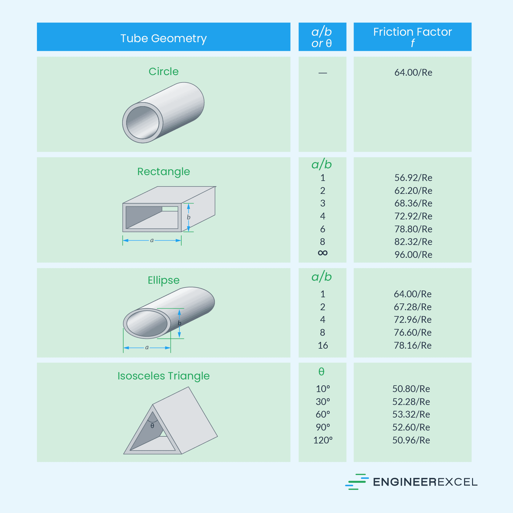
There are different equations to calculate the friction factor depending on the flow regime, however, its value is generally lower for laminar flow than for turbulent flow. The formula for calculating the friction factor of laminar flow in pipes of different cross sections are tabulated below.
Applications of Laminar Flow
In the industrial sector, laminar flow is key for efficient transportation of fluids in pipelines. By maintaining a smooth flow of liquids, you can minimize energy losses and reduce operating costs. This is particularly important in industries such as oil and gas, where efficient transportation of fluids is essential.
Laminar flow plays a crucial role in the design of many biomedical devices, too. For example, it is essential for artificial heart valves to mimic the natural flow of blood to minimize wear and tear. Additionally, in dialysis machines, laminar flow helps prevent clotting and efficiently removes toxins from the blood.
In the aerospace industry, achieving laminar flow over airplane wings and fuselage surfaces reduces drag and improves fuel efficiency. By carefully designing wing shapes and using innovative materials, you can minimize turbulence and optimize aerodynamic performance. This not only leads to cost savings, but also has a positive impact on the environment by reducing CO2 emissions.