
Friction losses happen when fluid flows through a conduit and encounters resistance from the internal surface of the conduit. In fluid mechanics, these losses are usually measured using dimensionless coefficients. In this article, we provide a list of the friction loss coefficients for various flow conditions and geometries.
What are Friction Loss Coefficients
Friction loss coefficients are dimensionless parameters that represent the energy loss due to friction within fluid systems, such as pipelines and ducts. They are primarily used in calculating pressure drop or head loss when designing fluid systems.

The resistance to fluid flow arises from factors like internal roughness of the conduit walls and other elements, like bends, fittings, and valves. The friction loss coefficients indicate the efficiency of the conduit in maintaining fluid energy as it moves through the system. A higher value denotes higher energy loss and, consequently, an increased pressure drop.
These coefficients depend on various aspects, including fluid characteristics, the material and roughness of the conduit, and the system’s geometry. Determination of friction loss coefficients involves experimental testing and analysis conducted by engineers.

Elevate Your Engineering With Excel
Advance in Excel with engineering-focused training that equips you with the skills to streamline projects and accelerate your career.
Different standards and equations utilize different friction loss coefficients, such as the friction factor in the Darcy-Weisbach equation and the C factor in the Hazen-Williams equation.
Friction Factor
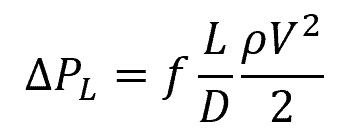
In the context of the Darcy-Weisbach equation, the friction loss coefficient would normally refer to the Darcy friction factor. The Darcy-Weisbach equation is a widely used formula for calculating pressure loss due to friction in pipe flow, as shown below:
Where:
- ΔPL = pressure loss due to friction [Pa]
- f = Darcy friction factor [unitless]
- L = pipe length [m]
- D = pipe diameter [m]
- ρ = fluid density [kg/m3]
- V = average flow velocity [m/s]
The friction factor depends on the characteristics of the fluid and the pipe or channel. Two primary factors influencing it are the Reynolds number, which represents the flow’s turbulence, and the relative roughness of the pipe material.
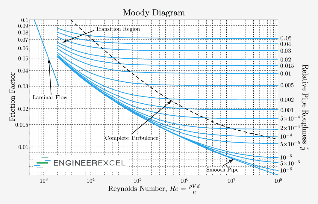
Various empirical formulas and charts are available for estimating the friction factor. The most famous one is the Moody chart, which offers a graphical representation of the relationship between Reynolds number, relative roughness, and the friction factor.
Alternatively, when dealing with laminar flow in a closed conduit, the friction factor can be computed using the Reynolds number. The table below lists the formulas for calculating the friction factor for various conduit geometries.

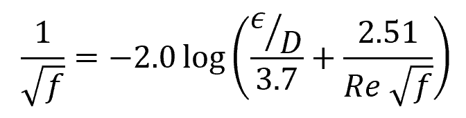
For turbulent flow, the friction factor can be calculated using the Colebrook equation:
Where:
- ε = average height of surface irregularities on the internal pipe wall [mm]
C Factor
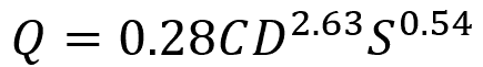
Another equation that relates frictional losses to flow rate is the Hazen-Williams Equation. In this equation, the friction loss coefficient would normally refer to the C factor or the Hazen-Williams coefficient, as shown below:
Where:
- Q = volumetric flow rate [m3/s or gpm]
- C = Hazen-Williams coefficient [unitless]
- D = pipe diameter [m or in]
- S = slope of hydraulic grade line [unitless]
Note that the slope of the hydraulic grade line is simply the head loss divided by the length of pipe.
In the Hazen-Williams Equation, the C factor represents the resistance to flow in a pipe due to friction, whose value primarily depends on the roughness of the pipe material. A higher C factor indicates a smoother pipe interior, which results in less friction and energy loss. Conversely, a lower C factor means the pipe has a rougher interior, causing increased energy loss due to friction.
The C factors for different pipe materials are listed in the table below.
The Hazen-Williams equation has an advantage over the Darcy-Weisbach equation in that its coefficient C is not dependent on Reynolds number, making it easier to use. In contrast, the Darcy-Weisbach equation is difficult to use due to the complexity of estimating friction factor.
The Hazen-Williams equation was widely used before computers became prevalent due to its simplicity, as it does not require a friction factor. However, it is only generally valid for water and does not account for temperature or viscosity, limiting its applicability to normal operating conditions. While it has been used for other non-corrosive and non-viscous fluids with similar properties to water, its accuracy may decrease for fluids with significant differences in density, viscosity, and other properties.