In the past, I’ve written about using the VLOOKUP function to pull data from tables into engineering calculations. However, you will probably find (if you haven’t already!) that as your spreadsheets become more sophisticated that VLOOKUP no longer gets the job done. For these situations, we can use Excel’s INDEX and MATCH functions to create even more powerful spreadsheet lookup tables.

INDEX Function

The INDEX function returns the value of a cell at a specified position within a range.

It’s syntax is as follows:

INDEX(array, row_num, [column_num])

Where:

• array is the range of cells from which you want to return a value. The data could be in a single row or column or multi-row/column table, but for our purposes we’ll just assume a single column.
• row_num is the row within the array containing the value you want to return
• column_num is a column within the array containing the value you want to return.

As an example, if we have a table of air properties at atmospheric pressure (source), we can use INDEX to return the 5^th value in the first column:

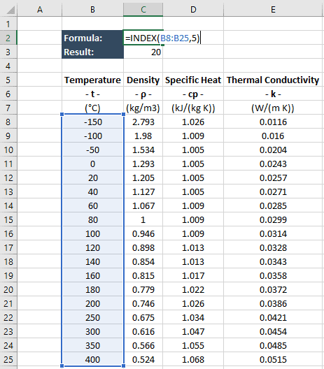
The function returns the value “20”, which is the fifth value in the selected array.

MATCH Function

Excel’s MATCH function returns the position of an item in a range.

The syntax is:

MATCH(lookup_value, lookup_array, [match_type])

Where:

• lookup_value is the value you want to find in the lookup_array
• lookup_array is the range of cells that Excel searches through to find the lookup_value
• match_type tells Excel how to match the lookup_value
  • If match_type = 1 (default value if omitted), Excel returns the greatest value less than or equal to the lookup_value. For this to work properly, the values in the lookup_array must be in ascending order.
  • If match_type = -1, Excel returns the smallest value greater than or equal to the lookup_value. For this to work properly, the values in the lookup_array must be in descending order.
  • If match_type = 0, Excel looks for a value that exactly matches the lookup_value. In this case, the lookup_array may be unordered.

Using the same air property data, we can use MATCH to tell us the position of the value “120” in the same array:

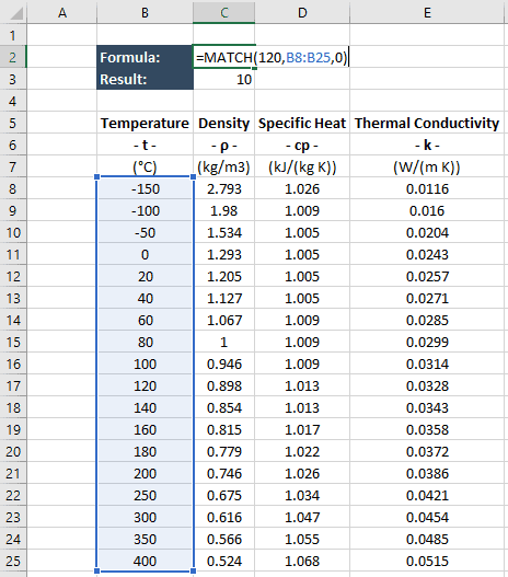
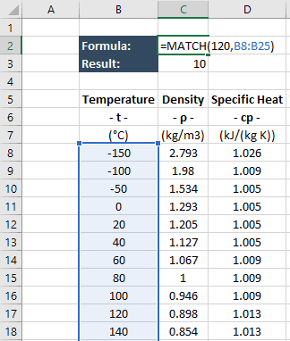
The function returns “10”, which is the position of the value “120” in the selected array. In this example, I set match_type=0 to specify an exact match. However, since an exact match exists in this case, omitting this argument would have given the same result.

Using Excel’s INDEX and MATCH Functions Together

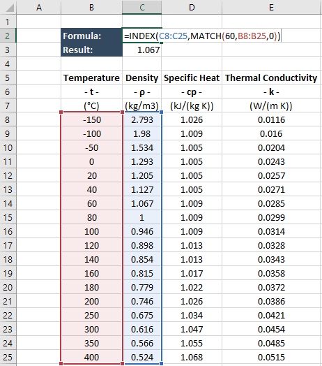
We can combine these two functions to do all the things that VLOOKUP can do (and more). If we want to find the density at 60 degrees C, we use a MATCH function for the “row_num” argument in the INDEX function instead of a static value.

Advantages

So why would we use INDEX and MATCH in place of VLOOKUP? Primarily, it’s because the combination of these two functions provides more flexibility and control than VLOOKUP.

Flexibility

VLOOKUP requires that the lookup array be the first column in a table of data. With INDEX and MATCH, lookup_array can be any column in the table. For instance, if we wanted to find the temperature that would reduce air density to 1 kg/m³, we would use the density column in the MATCH function, and the temperature data as the array in the INDEX function.

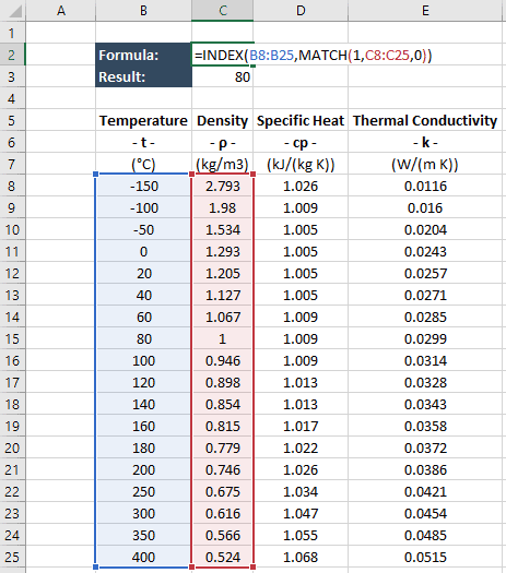
If we wanted to this with VLOOKUP, we would have to create a new table with the density data in the first row, or duplicate the temperature column to the right of the density column to obtain the same functionality.

Control

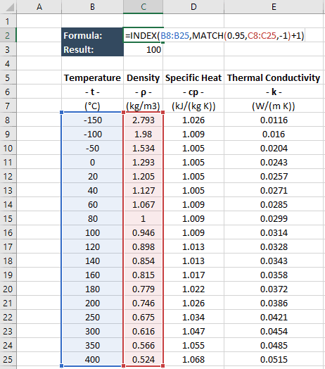
Another advantage that INDEX and MATCH provide over VLOOKUP is the control that you have, particularly when the lookup value does not perfectly match an entry in the lookup array or when the lookup array data is in descending order. As an example, let’s say we wanted to find the minimum temperature required to reduce the air density to less than 0.95 kg/m³. This data point doesn’t exist in the table, so the VLOOKUP function is useless in this situation.

We can use Excel’s INDEX and MATCH functions to perform this lookup, but because the data is in descending order we have to be careful. The only match_type argument in the MATCH function that will return any value is “-1”. However, this will return the position of the smallest value that is greater than or equal to 0.95, which is not what we want. We can get around this by adding “1” to the value returned by MATCH to offset one row down and get the correct value.

Wrap-Up

As you can see, Excel’s INDEX and MATCH functions can be used together to provide even more functionality than VLOOKUP alone.

Are you using these functions in any of your engineering spreadsheets? If so, tell me about it in the comments below!