INDEX and MATCH are great functions to use for flexible lookups of data in either 1D or 2D tables, but they can also be used to lookup data in 3D tables as well, where the output value “d” is a function of three inputs: a, b, and c. However, to use those functions in such a way, we need to use a few tricks to get the table ready.
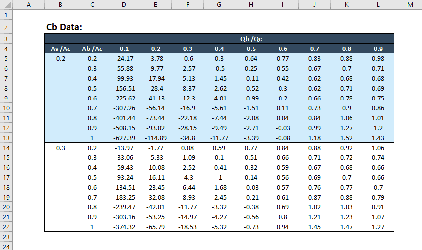
The table below was sent in to me by a subscriber to the EngineerExcel.com email list. It’s a table of coefficients for calculating flow in ductwork.
Preparing the 3D Table in Excel
As you can see, the value Cb is a function of three inputs:

Elevate Your Engineering With Excel
Advance in Excel with engineering-focused training that equips you with the skills to streamline projects and accelerate your career.
- As/Ac
- Ab/Ac
- Qb/Qc
The INDEX function can find data in a 2d table if we use both the row_num and column_num arguments. So, we could use this function to lookup the data if we first convert the table from 3D to 2D. Fortunately, it’s easy to do that in just three simple steps.
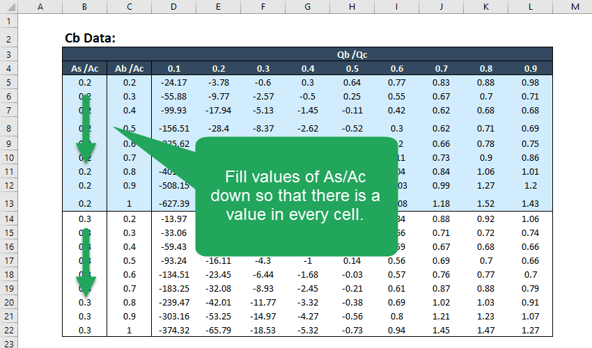
First, we’ll fill all the rows in the column labeled “As/Ac” with data.
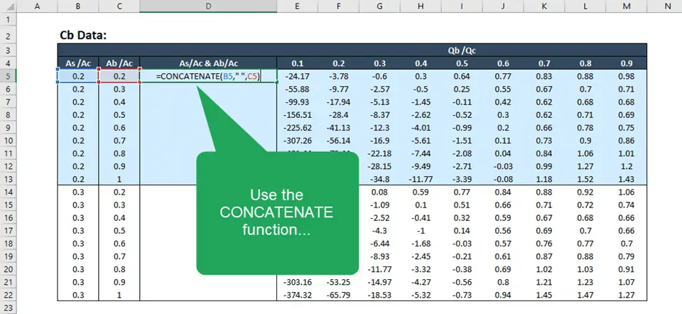
Then, insert a column to the right of the Ab/Ac values.
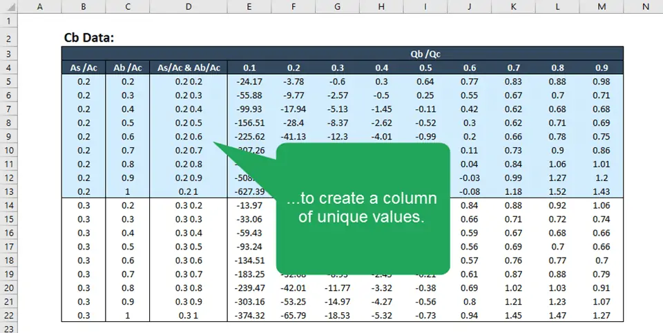
Finally, use the CONCATENATE function to combine the As/Ac values and Ab/Ac values into a single value in the newly created column. I also added a space between the values for clarity.
Looking Up Data from the 3D Table
Once we’ve converted the 3D table to one that has only two dimensions, with a unique value in column D for each row of Cb values, it’s a simple matter to use INDEX and MATCH to find the data.
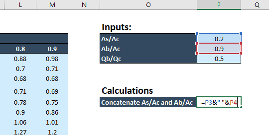
But first, we’ll need to set up the inputs by combining the input values for As/Ac and Ab/Ac into a single value that matches the column we just created. Again, we’ll use the concatenate function just like before.
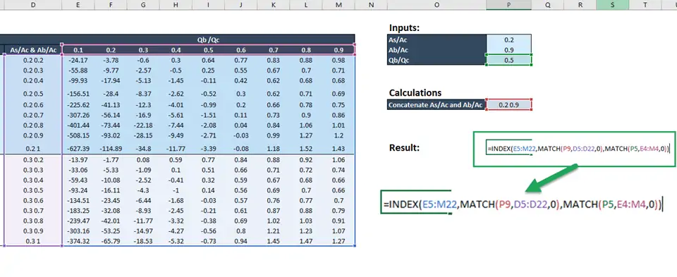
Finally, we can use the INDEX and MATCH functions to lookup the value of Cb from the inputs Qb/Qc and the combination of As/Ac and Ab/Ac. Since the table has two dimensions (horizontal and vertical), we’ll use both the row_num and column_num arguments. The syntax of the function is like this:
=INDEX(Cb_values,MATCH(value_on_vertical_axis,vertical_array,0),MATCH(value_on_horizontal_axis,horizontal_array,0)
The final argument of “0” in the MATCH function will return an exact match only.
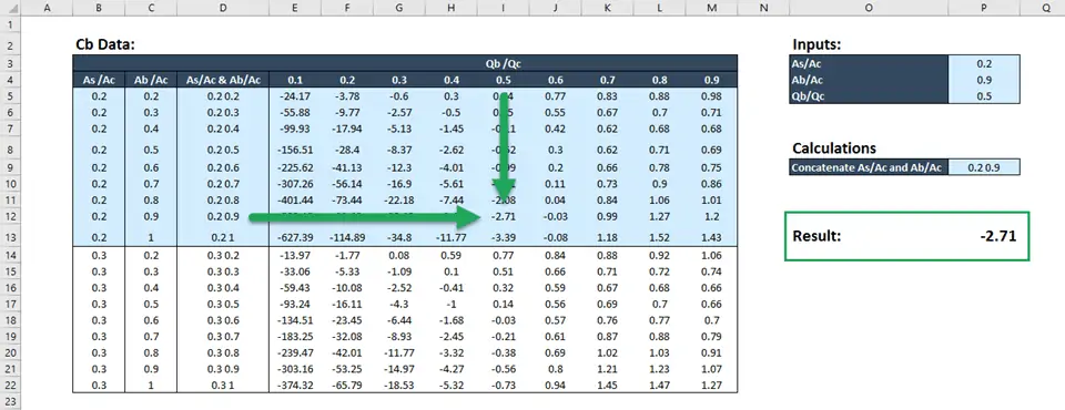
The resulting value is -2.71. Of course we can check the table to be sure that we have the intended value:
Wrap Up
So that’s how you can look up data from a 3D table in Excel. What’s great about this technique is that it can even be expanded to n-dimensional tables. The key is to convert the table to two dimensions by creating a column (or row) of unique values that can be found using the INDEX and MATCH functions.
