
It’s easy to calculate a slope in Excel using the SLOPE function, but it’s also possible to use chart trendlines and simple arithmetic as well. This article will show you how to do all three, so keep reading!
with the
: How to without a
The uses to calculate the of in without creating a , adding a , or performing complex .
The syntax of the is shown below:
=SLOPE(known_ys, known_xs)

Elevate Your Engineering With Excel
Advance in Excel with engineering-focused training that equips you with the skills to streamline projects and accelerate your career.
where:
known_ys: the -values (the values on the vertical axis or dependent variables)
known_xs: the -values (the values on the horizontal axis or independent variables)
Examples
The can calculate the when there are 2 or more -values and 2 or more -values.
Example 1
In this example, there are only two x-values and two y-values. The for calculating the between the two points defined by the x- and y-values is
=SLOPE(C3:C4,B3:B4)
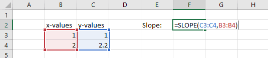
The result is 1.2.
Because there are only two values, the slope could have been calculated as the rise over the run, or the difference in the y-values divided by the differences in the x-values.
=(C4-C3)/(B4-B3)
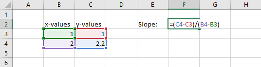
Of course, the result of this calculation is also 1.2.
Example 2
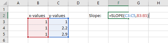
If there are more than two pairs of x- and y-values, the SLOPE function returns the slope of the line of best fit for the dataset. Let’s see how it works by adding another pair of x- and y-values to our data from before. Now the formula is:
=SLOPE(C3:C5,B3:B5)
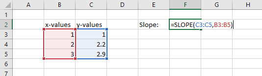
Here the result is 0.95.
This is not the slope between any two sets of points. Instead, it is the slope of a straight line that “best fits” the data. The slope of the best fit line is calculated using linear regression.
SLOPE Function Errors
#DIV/0! Error: Only One Pair of Values Selected
If only one pair of x- and y-values is selected as the SLOPE function arguments, this equivalent to trying to calculate the slope of a single point. This is undefined, and so the result is a #DIV/0! error
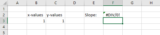
In the example below, one x-value and one y-value are entered as arguments.
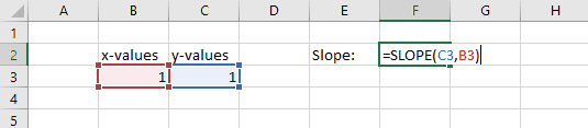
Because the “run” is zero, a #DIV/0! error is returned:
#DIV/0! Error: Data Points Represent a Vertical Line
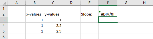
When all x-values in the dataset are the same, the line represented by the data is perfectly vertical. The slope is infinite or undefined in this situation because the “run” in the denominator is zero. This also causes a #DIV/0! error, as demonstrated below:
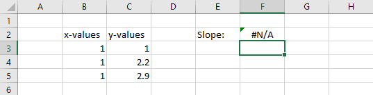
#N/A Error: Different Number of X- and Y-values
An #N/A error can occur with the SLOPE function in Excel when the number of y-values differs from the number of x-values. In the example below, 3 x-values are chosen as arguments for the SLOPE function, but only 2 y-values are chosen.
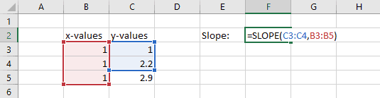
This returns an #N/A error:
How to Find the Slope of a Trendline in Excel: Find Slope on an Excel Scatterplot
Charts are a great way to visualize a data set, and they also provide an opportunity to add a trendline that can display the slope of a set of x- and y-values.
Step 1: Graph the Data
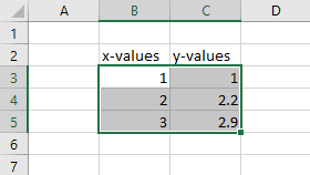
The method below works if the data is on a spreadsheet with the x-values in one column and the y-values in another column immediately to the right of the x-values as shown in the images below.
Select ALL the data…
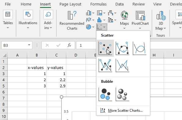
…then insert a scatter chart by selecting Insert > Scatter Chart. (The scatter chart with only data markers works best for this.)
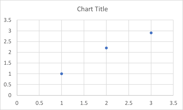
The data will be shown on a chart like this:
Step 2: Add a Trendline
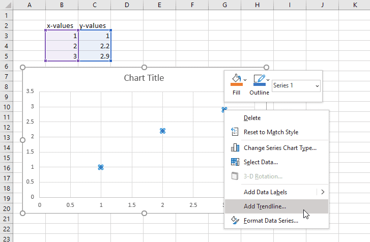
Next add a trendline by right-clicking on the data series and selecting “Add Trendline…”
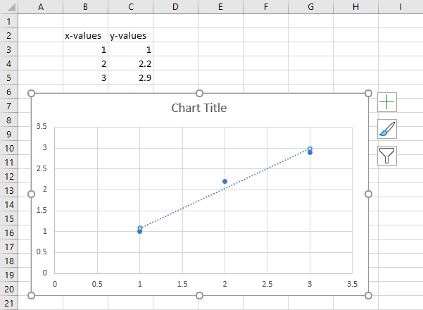
This adds a linear trendline to the chart by default:
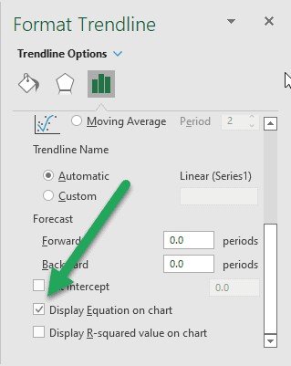
Step 3: Display the Trendline Equation on the Chart
To determine the slope, display the equation on the chart by selecting “Display Equation on the chart” in the “Format Trendline” pane that appears on the right side of the screen:
The trendline equation is displayed on the chart:
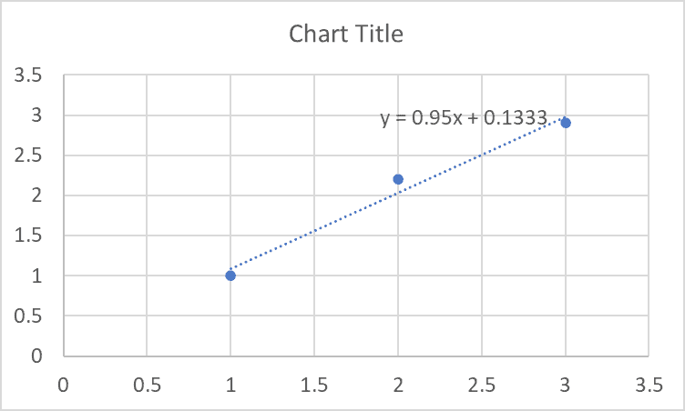
The slope is the coefficient in front of x, or 0.95.
How to Calculate Rise over Run in Excel
As discussed above, if there are only two x- and y-values, it possible to calculate the slope, or rise over run, of the data points without using the SLOPE function.
Rise over run is the difference between the y-values (rise) divided by the difference in the x- values (run).
When using this method, it’s important to be consistent in the order of the x- and y-values in the evaluation. If the rise is calculated as the second y-value minus the first y-value, the run must be calculated as the second x-value minus the first y-value.
In the example below, the rise over run is calculated by
=(C4-C3)/(B4-B3)

The rise over run is 1.2.
Calculate Slope in Excel with the LINEST Function
The LINEST function is an array function that can be used to perform linear regression and non-linear curve fitting. However, it can calculate both the slope and the intercept of a data set with a single formula.
The LINEST function has similar arguments to the slope function, with a couple of additions:
=LINEST(known_ys,known_xs,const,stats)
where
known_ys: the known y-values
known_xs: the known x-values
const: (optional) if TRUE, the y-intercept is calculated normally, if FALSE the y-intercept is set to 0
stats: (optional) if TRUE, additional regression statistics will be returned, if FALSE no additional statistics are returned
In the example below, the same x- and y-values are chosen. CONST is TRUE so that the y-intercept will be calculated normally, and STATS is FALSE so that no additional statistics are returned.
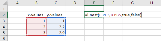
In Excel 365 LINEST is a dynamic array and the results are returned to two cells. The first cell contains the slope and the second cell contains the y-intercept. (If you are using a version of Excel other than Excel 365, only the slope will be returned.)
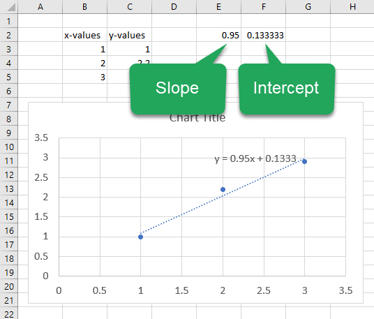
The values of the slope and intercept returned by LINEST match the values in the chart trendline. The slope is 0.95 and the y-intercept is 0.133