
A Gaussian function has many different purposes in engineering although most people probably recognize it as a “bell curve”. Most commonly, it can be used to describe a normal distribution of measurements. Sometimes it’s necessary to fit a Gaussian function to data, so this post will teach you how to perform a Gaussian fit in Excel.
Below is a set of tank temperatures and the number of times they have been observed (occurrences).
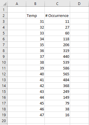
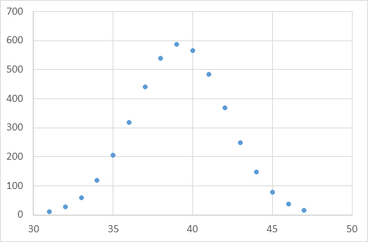
When we plot them (with temperature on the X-axis and # of occurrences on the Y-axis), we can easily see the characteristic bell-curve shape.
Finding the Gaussian Fit in Excel

Elevate Your Engineering With Excel
Advance in Excel with engineering-focused training that equips you with the skills to streamline projects and accelerate your career.
To find the Gaussian fit in Excel, we first need the form of the Gaussian function, which is shown below:
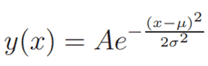
where A is the amplitude, μ is the average, and σ is the standard deviation.
If we want to determine these coefficients from a data set, we can perform a least-squares regression.
For many non-linear functions, we can convert them into a linear form and use the LINEST function to determine the coefficients of the best-fit curve.
However, that isn’t an option for this function (or at least I’m too lazy to work through the math :)) so we are going to use a different method to find the coefficients using Solver instead.
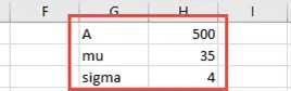
The first step is to make a guess at the coefficients in the Gaussian function. Don’t worry about how good your guess is for now.
Next, create a new column for the Gaussian function using the coefficients that were entered previously.
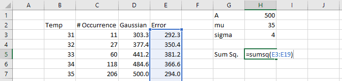
Enter the Gaussian function in the cell at the top of this column. In this case, the x’s are the temperature bins. My data started at cell B3, so the cell formula is as follows:
=A*EXP(-((B3-mu)^2)/(2*sigma^2))
Watch your parentheses here! They can be tricky.
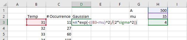
In my spreadsheet, I’ve created names for the cells containing the coefficients. This is completely optional, but it makes the cell formula easier to understand.
Next, we need to find the value of our Gaussian function for each of the temperature bins, so fill the cell down so that it fills the entire column. (A quick shortcut is to hold down the Shift key and double click the square in the lower right corner of the cell. This will automatically fill the formula down to the exact length of the adjacent column.)
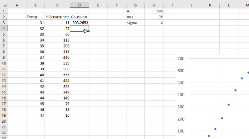
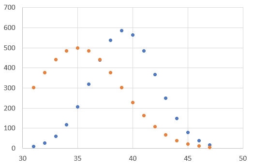
If we plot the function (orange) and the data (blue) on the same chart, we can see that the initial coefficient guesses are way off!
No worries. We can use Solver to find the optimum values of the coefficients that minimize the error between the data and the Gaussian function.
To do this, we will calculate the error between the occurrences predicted by the Gaussian function and the occurrences in the data. When we’ve found coefficients that minimize the overall error for all of the data points, we’ll have found the best-fit coefficients. This technique is called least-squares regression.
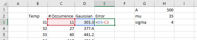
To perform least-squares regression in Excel, create a column to calculate the difference (error or residuals) between the Gaussian function and the data.
In a separate cell, calculate the sum of the error values squared using the SUMSQ function.
=SUMSQ(E3:E19)
Now, the fun part – we’re going to use Solver to “automagically” find the coefficients to achieve the best Gaussian fit.
Using Solver to Fit a Gaussian Function in Excel
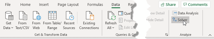
You can access the Solver add-in on the far-right side of the Data tab.
If you’ve never used the Solver add-in before, you’ll need to activate it. I’ve already put together a detailed post showing how to enable the Solver add-in here. Go through that exercise first, and come back here once you’ve enabled the add-in.
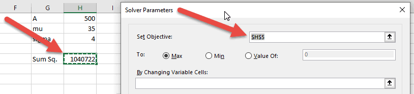
With the cell containing the SUMSQ function selected, open the Solver add-in. (By selecting it before opening Solver, it will automatically be set as the “Objective Cell”, or the cell we want to optimize.)
There are a lot of options in this add-in, but we only need to use a few.
First, make sure the option to minimize the Objective cell is selected. After all, we want to minimize the difference between the prediction and the actual data.
Next, select the variable cells. These are the cells containing the values of the coefficients.
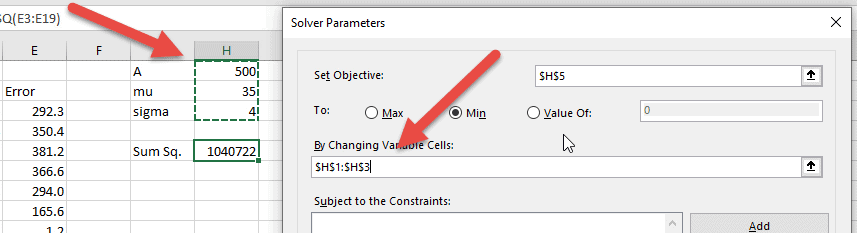
So now we’ve told Solver to minimize the sum of the squared errors (or residuals) by changing the Gaussian function coefficients.
All that’s left to do is click “Solve”, and Solver will quickly find the optimum coefficients.
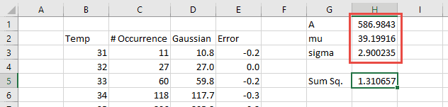
Gaussian Curve Fit Result
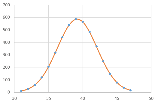
After changing the function series to a line, we can see that the Gaussian function now matches the data well. Further, we can confirm that the errors at each temperature are very small.
So that’s how to do a Gaussian fit in Excel. I hope this helps.
Oh, and by the way, you can use Solver in this same way to determine the coefficients of the best-fit curve for any function you can dream up. Give it a try!