
In the last section, you saw how to do a basic text import. The Text Import Wizard offers a lot of options to customize this type of import. You can specify how you’d your text data to be imported, minimizing the amount of cleanup that you need to do on the data.
In this section, we’ll use Ideal_Gas_Property_Data.txt as the data source. Go to Data > Get External Data > From Text, and open that file. The first window of the Text Import Wizard will open.
There are two main types of data files that you’ll import into Excel. Delimited files have a character separating the columns (i.e. a tab stop). Fixed width files have a specific number of characters in each column.
First, we’ll see how this data looks with the Delimited option. Choose it, then click Next.
Delimiters can be virtually any character. Tab, comma and space are the most common. The tab character is selected by default. However, in the preview window, there are no black lines separating the column – this tells us that Excel hasn’t found any tab delimiters. Unselect Tab, and choose Space. Now, black lines will appear between the columns:

Elevate Your Engineering With Excel
Advance in Excel with engineering-focused training that equips you with the skills to streamline projects and accelerate your career.
Excel recognizes that the columns of data are separated by spaces. It automatically checks the box for “Treat consecutive delimiters as one.” In this text file, there are multiple spaces between the columns of data. If this box was not checked, each space would indicate a new column.
Click Next, then Finish. Choose a location on the worksheet to store the data and click OK.
Viewing the data in the spreadsheet exposes a flaw in selecting the space delimiting option. Gas names such as “carbon dioxide” and “carbon monoxide” are composed of two words separated by a space. Excel interprets this space as a column separator, so those rows have an extra column and all of the data is shifted:
Although we could manually clean up the data, those changes would be lost if the data were refreshed.
Instead, we’ll choose better options in the Text Import Wizard. Right-click on the data and select Edit Text Import.
Next, double-click on the file Ideal_Gas_Property_Data.txt.
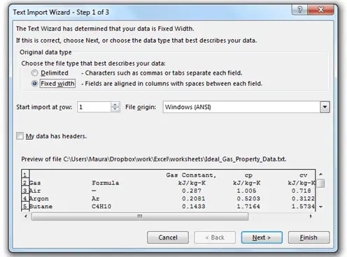
This time, instead of the Delimited option, choose Fixed width. Click Next. Excel will automatically determine where the columns should be, and places break lines as separators between them. To move a break line, click and drag it to a new position.
You can also add or remove break lines. To add one, click at the top of the preview window, below the ruler (where the arrowheads are showing for the existing break lines). To delete one, double-click on it, or drag it away from the preview window.
Don’t worry about any excess spaces before or after an entry. Excel will clean those up. Just adjust the break lines so that each column includes all of the intended data. In this case, the defaults are fine. Click Next.
The third window of the Text Import Wizard contains options to set a data format for each column. The General format is appropriate for most data. It treats numeric values as numbers, date values as dates, and everything else as text. You can also specify a date or text format. Click each column in the preview window and set its type.
You also have the option of omitting columns. Sometimes, data files contain more information than you need. You can select any of these columns and choose Do not import column (skip) to remove it from the data table. For example, if you only need the columns containing the gas name and the constant pressure specific heat, you can remove the other columns. Select the Formula column, then click Do not import column (skip). The header will change from “General” to “Skip Column” (see the headers in the image below). Repeat for the other unnecessary columns.
Click Finish, and you’ll have a table containing only the pertinent data, with no additional cleanup required.