One of the things that makes Excel such a great tool is the ease at which you can automate certain tasks.
This creates many opportunities for engineers to save time and prevent errors.
One often-overlooked opportunity for automation is in chart titles and axis titles.
Excel allows you to link the title of a chart or axis to a cell so that the title automatically updates whenever an input or results cell changes.
Create an Excel Chart with Dynamic Chart Titles
The first step, of course, is to create the chart.

Elevate Your Engineering With Excel
Advance in Excel with engineering-focused training that equips you with the skills to streamline projects and accelerate your career.
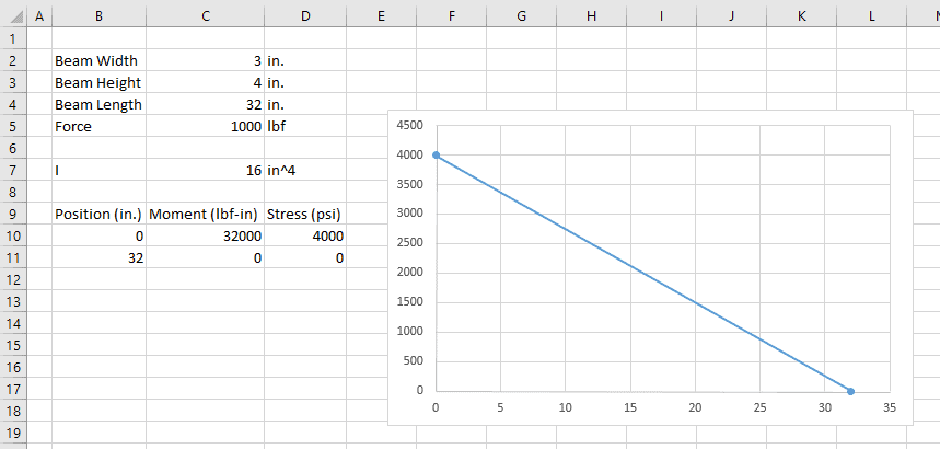
In this example I’ve created a chart of bending stress in a cantilevered beam with a rectangular cross-section.
The cross-sectional width, height, and length as well as the point load are all variables in the worksheet.
I calculated the moment of inertia and the bending stress at both ends of the beam.
The chart is just a simple scatter plot of the stress results vs position.
Create an Excel Chart Title Formula with Concatenate
I wanted the title to reflect the dimensions of the beam as well as the load applied so that these items would be documented with the chart.
That way in case the chart is ever copied and pasted into an email, Word document, or PowerPoint presentation the inputs to the calculations will be known.
The CONCATENATE function can be used to create a descriptive title in a cell on the worksheet. Then that cell can be used as the chart title.
Returning to the worksheet, I entered the following formula into cell G3:
=”Bending Stress Diagram: “&C2&” in. W x “&C3&” in. H, “&C5&” lbf”
The formula result was:
Bending Stress Diagram: 3 in. W x 4 in. H, 1000 lbf
This string of text does everything I wanted the chart title to do – it contains both a description of the data in the chart, as well as information about the beam dimensions and applied load.
Create an Excel Chart Title from a Cell
The final step was to specify the result of this formula as the chart title. Excel makes this easy.
First, select the default chart title.
Next, click inside the formula bar and type in an “equal” sign (=).
Finally, select the cell containing the chart title and hit Enter.
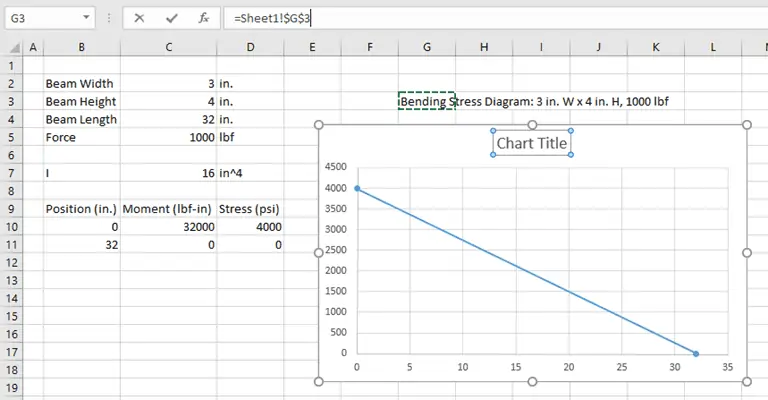
That’s it – the formula result is now used as the title of the chart.
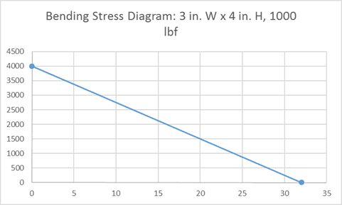
I did a few other things as best practice – like adding axis labels and resizing the chart title so that it fits on one line.
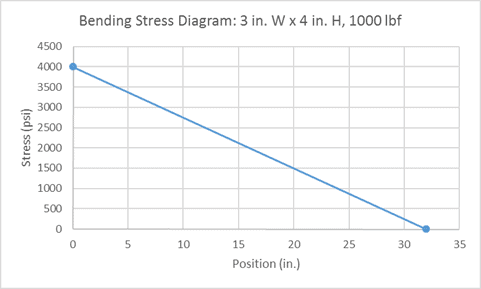
Note: The axis labels can be made to update dynamically using the same method as well. (Although for this example it wasn’t necessary.)
Update a Dynamic Chart Title in Excel
So what happens when the inputs change?
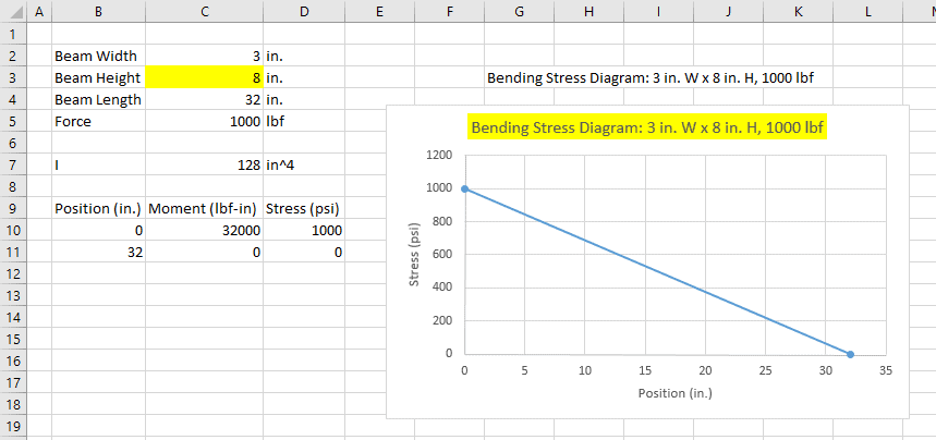
When I changed the beam height to 8 inches, the stress results updated AND the title of the chart also changed to reflect the new beam dimensions.
