Continuity Equation: A Complete Guide

The continuity equation describes the conservation of some quantity w that is being transported within a system.

The Continuity Equation

In general, the continuity equation can be written as:

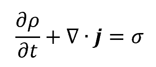
where:

• ρ is the quantity w per unit volume, i.e., the volume density of w
• j is the flux of quantity w
• σ is the generation or removal of w

Specifically, the continuity equation states that the change in the amount of w can be determined by how much flows through a system boundary and how much is gained or lost by sources and sinks, respectively, inside the boundary.

Flux

The flux of a system specifies the amount of quantity w that flows through the system per unit time per unit area. The system flux may describe the flow of mass or energy. To calculate the flux, the surface integral is used. With regard to continuity, a small volume element defined by Δx, Δy, and Δz has a lateral surface area of ΔA, as shown in the following figure:

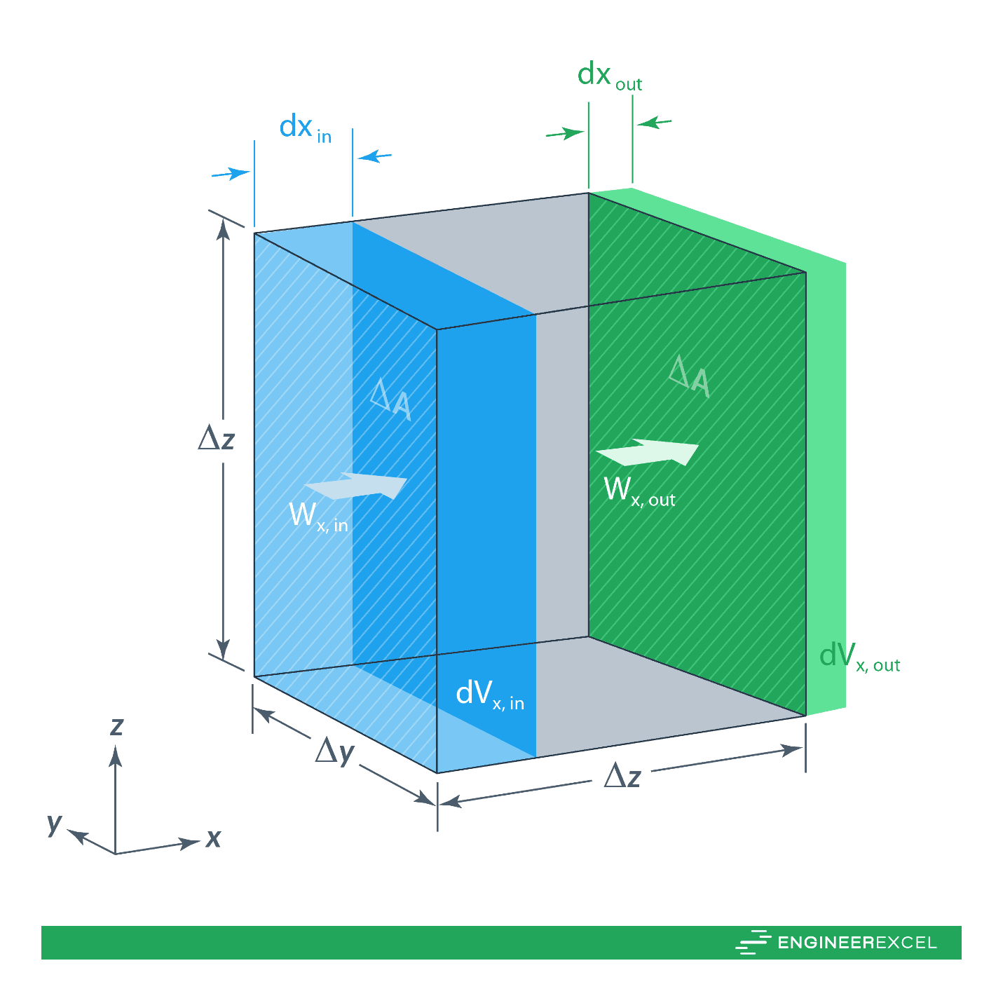
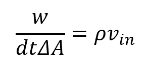
For quantity w flowing in the x-direction, over time dt, dw_in enters the system and dw_out leaves the system. If w is flowing with a velocity of v_in, over time dt it will travel dx_in. Therefore, the volume in dV­_in is equal to dx_in times ΔA. Mathematically, this can be expressed as follows:

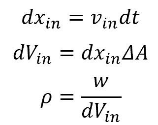
Combining and simplifying the above equations yields a simplified formula for the flux:

Taking the limits as Δx, Δy, and Δz go to zero yields:

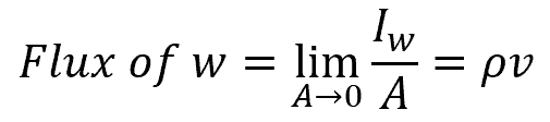
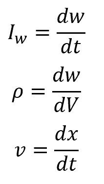
where:

Fick’s Law

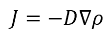
Fick’s Law states that the flux will move from a region with a high volume to a region with a low volume and that the magnitude of the flux is proportional to the concentration gradient. It is expressed mathematically as:

Substituting the continuity equation yields:

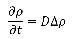
where:

• ∆=∇², i.e., the Laplace Operator
• D defines the diffusivity

In general, diffusion describes the movement of something from a high concentration to a low concentration.

Applications Of The Continuity Equation

Having defined a general form for the continuity equation, its application to various engineering applications is discussed in the following.

Continuity Equation for Fluid Mechanics

The most common application of the continuity equation is to fluid mechanics. In this field, the continuity equation describes the conservation of mass. Specifically, it states that the mass leaving a system is equal to the mass entering the system plus the accumulation of mass within the system due to sources and sinks. Mathematically, this is expressed as follows:

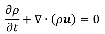
where:

• ρ is the density of the fluid, with units of lbm/ft³
• u is the fluid flow velocity vector field, with units of ft/s

For incompressible fluid flow, the density does not change, so the continuity equation for fluid mechanics applications can be simplified to:

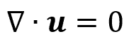
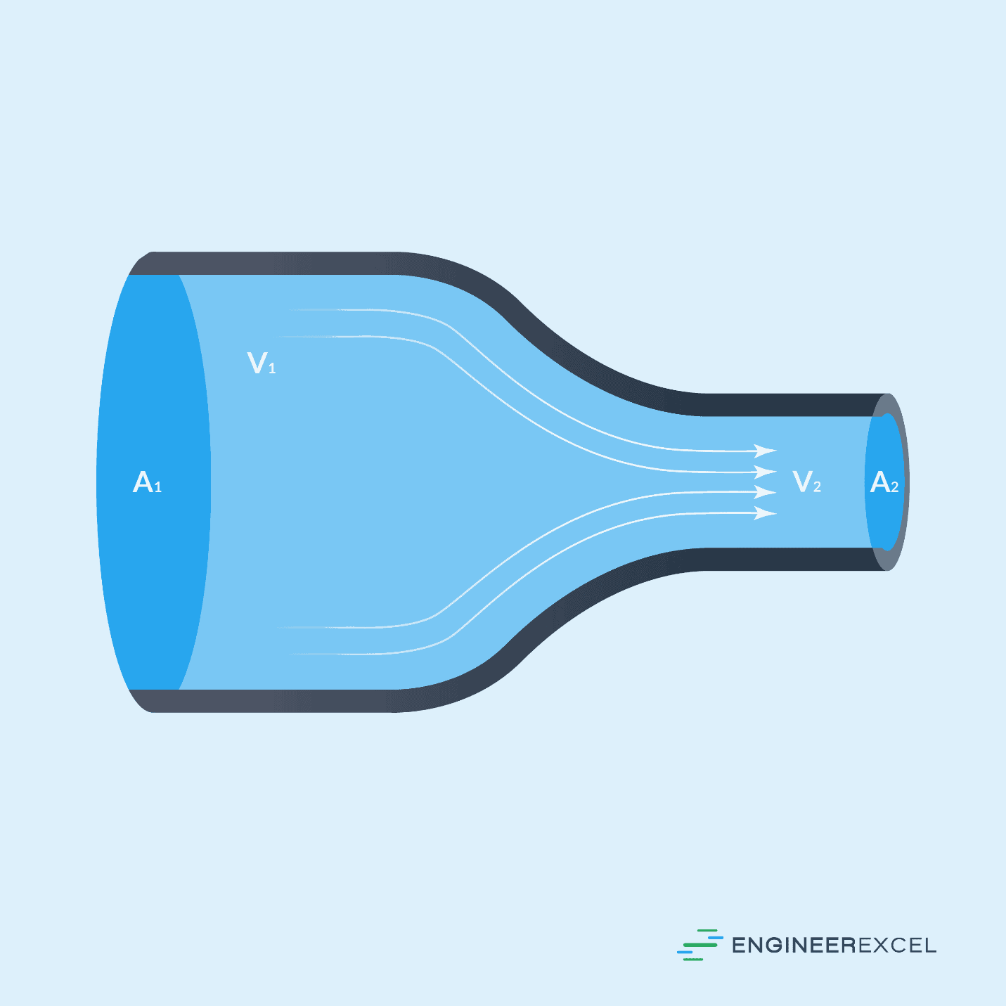
The above equation may be recognized as one of the Navier-Stokes equations. This specifies that the divergence of the velocity field is zero throughout the system. In other words, because the local volume dilation rate is zero, the velocity of an incompressible fluid (such as water) flowing through a converging pipe will increase.

A simplification of the continuity equation for fluid mechanics is:

where ṁ is the mass flow rate, with units of lbm/ft3s. The mass flow rate can also be expressed as:

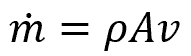
The following figure shows this expression of the mass flow rate and the continuity equation:

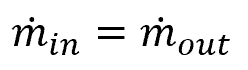
If a system has multiple inlets and outlets, the sum of the inlets will be equal to the sum of the outlets, as follows:

Fluid Mechanics Example

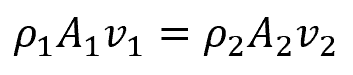
For the flow of water (density of 62.4 lbm/ft³) through a pipe that increases in diameter from 7 in to 12 in, if the flow velocity is 27.8 ft/s at the inlet, the flow velocity at the outlet can be calculated as follows:

The above can be expanded as follows:

Solving for v₂:

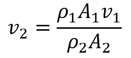
Because water is incompressible, ρ₁ = ρ₂, therefore,

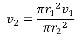
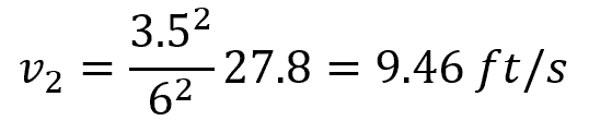
Substituting values:

Continuity Equation for Electromagnetism

The continuity equation may also be applied to electromagnetic applications to describe the conservation of electric charge within a system. Specifically, it states that the divergence of the current density J is equal to the negative rate of change of the charge density. Mathematically, this is expressed as follows:

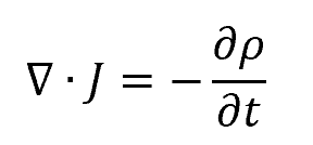
where:

• J is the current density, with units of amps per unit area, i.e., A/ft² in standard units
• ρ is the charge density, with units of coulombs per unit volume, i.e., C/ft³ in standard units

Because an electric current is the movement of a charge, in electromagnetic applications the continuity equation states that the charge moving out of a system (positive current density divergence) will decrease the overall charge of the system, therefore, the rate of change of the charge density is negative and the charge of the system is conserved.

The continuity equation for electromagnetic applications can be simplified as follows:

where Q̇ is the charge flow rate, with units of C/ft³s.

Electromagnetism Example

For a body with a charge of +10Q placed near another body with no charge, the continuity equation states that the charge will be equally divided between both bodies such that each has a charge of +5Q. This is shown in the following figure:

Continuity Equation for Thermodynamics

In thermodynamics applications, the continuity equation describes the conservation of energy. Specifically, it states that the energy (in the form of heat) flowing out of a system is equal to the energy flowing into the system. Mathematically, this is expressed as follows:

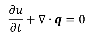
where:

• u is the local energy density, with units of energy per unit volume, i.e., Btu/ft³ in standard units
• q is the energy flux, with units of energy transferred per unit area per unit time, i.e., Btu/ft²s in standard units

Although heat (energy) cannot be created or destroyed in a system, internal system heat sources, such as friction, may increase the temperature of the flow leaving the system.

The continuity equation for thermodynamics applications can be seen in the first law of thermodynamics:

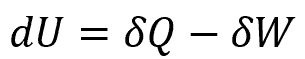
where:

• dU is the change in the internal energy of a system, with units of Btu/s
• δQ is the energy added to a system through heating, with units of Btu/s
• δW is the energy lost from the system due to work done by the system, with units of Btu/s

Note that the heat and work are not defined as specific processes, and are only defined based on the specifics of a scenario. For example, the heating of a system, δQ, may be defined as:

where:

• T is the temperature, with units of °F
• dS is the change in entropy of the system, with units of Btu/°F∙s

The work of a system, δW, may be defined as:

where:

• P is the system pressure, with units of lbf/ft²
• V is the system volume, with units of ft³

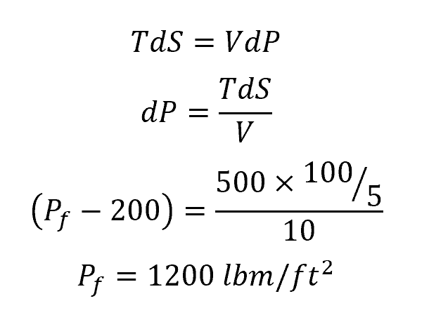
Applying the continuity equation, the internal energy of the system does not change, so

Thermodynamics Example

For a system at a pressure of 200 lbf/ft² subject to a 500°F heat source whose entropy changes by 100 Btu over a period of 5 s, if the system volume remains constant at 10 ft³, the change in system pressure can be calculated using the continuity equation as follows: