
The Colebrook-White Equation (or simply Colebrook Equation) is an engineering equation used to approximate the Darcy friction factor (or Darcy-Weisbach friction factor) for turbulent flow in full flowing pipes or ducts. The friction factor is required to calculate the pressure drop or head loss due to wall roughness using the Darcy Weisbach equation.

where
- f is the Darcy friction factor
- ε is the pipe roughness height
- Dh is the hydraulic diameter (for full flow)
- Re is the Reynolds number
It’s important to note that the Colebrook Equation is only valid for turbulent flow in pipes, where the Reynold’s number is greater than ~4000. The Reynolds number is influenced by the pipe flow velocity, pipe diameter, and kinematic viscosity of the fluid.
There is also a form of the equation for free surface flow in channels:

Elevate Your Engineering With Excel
Advance in Excel with engineering-focused training that equips you with the skills to streamline projects and accelerate your career.

In the free-surface form R is the hydraulic radius.
Colebrook Equation Calculator
The above calculator uses the Haaland equation, an explicit approximation of the Colebrook equation, to calculate the friction factor.
How to Solve Colebrook Equation for f
The Colebrook equation is an implicit equation. That means there is no way to arrange the equation to get the Darcy friction factor on one side of the equal sign.
Therefore, iteration is required to solve the Colebrook equation.
How to Solve the Colebrook Equation by Hand
Water is flowing through a pipe with a roughness height of 0.00005 meters, a hydraulic diameter of 0.025 meters. The Reynolds number of the flow is 6000. Calculate the Darcy friction factor.
Because the Reynolds number is greater than 4000 the flow in the pipe is turbulent, so the Colebrook equation can be used to calculate the pipe friction factor.
Step 1: Rearrange the Colebrook equation into the form:

Step 2: Choose a guess value for f
Since the values of f range from 0.01 to 0.1, choose a value of 0.05 which is approximately the mean value of f.
Step 3: Solve the right-hand side of the equation
Input the values for ε, Dh, and Re along with the guess value for f and calculate the result:

Step 4: Check the accuracy of the solution
Since the calculated value of f does not match the guess value of f, we need to continue iteration.
Step 5: Use the new value of f in the right-hand side of the equation and recalculate

Step 6: Repeat iteration until the guess value of f matches the calculated value
The process above is continued until there is an approximate match between the guess value of f and the calculated value. The table below shows the progression of iterations:
| Iteration Number | Friction Factor Guess | Friction Factor Result |
| 1 | 0.05 | 0.03648 |
| 2 | 0.03648 | 0.03803 |
| 3 | 0.03803 | 0.03782 |
| 4 | 0.03782 | 0.03785 |
On the fourth iteration, the friction factor guess matches the friction factor result to 3 decimal places, therefore 0.0378 is a reasonable approximation of the friction factor.
How to Solve the Colebrook Equation by Calculator
Most graphing calculators have built-in capability to solve equations. Using this functionality, you can enter the equation into your calculator with friction factor as a variable, and solve for f. The video below shows how to use the solver function on a graphing calculator to solve an equation.
How to Solve Colebrook Equation in Excel
In Microsoft Excel, the Colebrook equation can be solved using Goal Seek. If the value of f is contained in a cell, Goal Seek automatically adjusts that value until an objective is met in another cell. By setting the objective to a target value of zero, Excel will iterate on the value of the friction coefficient. The iteration will continue until an estimate is found that reduces the error between the objective and the target to an acceptable level.
- Enter an initial guess value for f in cell A1
- Enter the left side of the equation with A1 as an input in cell A2
- Enter the right side of the equation with A1 as an input in cell A3
- In cell A4 (the objective cell) enter the following formula: =A3-A2
- Use Goal Seek in Excel to find the value of A1 that makes A4 equal to 0
How to Solve Colebrook Equation using VBA
To solve the Colebrook equation using a root-finding VBA subroutine is required. Bisection, False-Position, or the Secant Method are all valid algorithms. The root-finding subroutine can be used in conjunction with a user-defined function containing the Colebrook equation rearranged with all the terms on one side of the equal sign.
The VBA root-finding subroutine guesses at the value of f and calls the user-defined function to check the guess. If the guess is not within an acceptable level of error, the algorithm will refine the guess. it will then recheck the guess and iterate as many times as required to find the value of the friction factor that is produces an acceptable level of error in the VBA user-defined function.
Colebrook White Equation Derivation and History
The Colebrook white equation was not derived from first principles, rather it was developed based on curve fitting to empirical data. C.F. Colebrook and C.M. White performed their research on the topic of friction factors for turbulent fluid flow in England during the late 1930’s and Colebrook published his paper introducing the equation in 1939 in the Journal of the Institution of Civil Engineers, Volume 11.
Colebrook Equation vs. Darcy Weisbach Equation and Darcy Friction Factor
Typically, the Colebrook Equation is used to estimate the Darcy-Weisbach friction factor, f. The friction factor can then be input into the Darcy-Weisbach equation to calculate the pressure drop in a pipe if velocity is known or velocity if pressure drop is known.
The Darcy- Weisbach equation is shown below:

where:
- Δp is the pressure loss due to friction
- L is the pipe length
- f is the Darcy friction factor
- ρ is the fluid density
- v is the average flow velocity
- D is the hydraulic diameter
It’s also possible to rearrange the Darcy-Weisbach equation to solve for the friction factor if the other inputs are known:

The Darcy-Weisbach equation is universally valid for steady-state flows in pipes and ducts that are incompressible.
Colebrook Equation vs. Moody Diagram
Prior to the widespread use of computers and calculators that could be used to solve the implicit Colebrook equation, an easier method of estimating the pipe friction factor was required.
Lewis Moody solved the Colebrook equation to create what is known today as a Moody Diagram or Moody Chart. Since three values (pipe roughness, diameter, and Reynolds number) must be known to calculate the friction factor, Moody combined the dimensional terms of roughness and pipe diameter into a single value called relative roughness, or the ratio of pipe roughness to pipe diameter, ε/D. The Moody diagram contains curves for many values of relative roughness plotted against the Reynolds number.
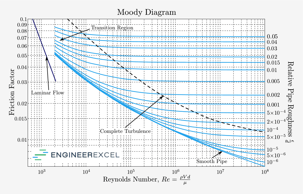
To find the friction factor on a Moody chart:
- Calculate the value of the relative roughness from the roughness and diameter
- Find the appropriate curve for the relative roughness on the Moody diagram
- Find the point where the friction factor curve intersects the Reynolds number
- Estimate the friction factor by finding the value on the vertical axis that is directly to the left of the point where the Reynolds number and friction factor curve intersect
A downside of the Moody diagram is that it is inconvenient for automated calculation of friction factor and pressure drop using computer programs or spreadsheets. That is why it can be valuable to solve the Colebrook equation.
Colebrook Equation Approximations
Because the Colebrook equation is an implicit equation and cannot be solve directly for f, several explicit equations have been proposed that allow f to be calculated direction. The most common are the Swamee-Jain Equation and Haaland Equation. Both approximations are for full flow in a pipe.
Since they are approximations of the Colebrook equation, they will not return the exact same results. However, it’s important to remember that the Colebrook equation itself is based on fitting to empirical data.
Swamee Jain Equation
The equation developed by Swamee and Jain in 1976 can be used to calculate the friction factor directly:

The friction factor calculated from the Swamee-Jain equation matches the Colebrook equation to within 1.0% for relative roughness between 10-6 and 10-2 and Reynolds number between 5000 and 108
Haaland Equation
Haaland’s equation, first proposed in 1983, is another method for estimating the friction factor that has an explicit form and can be solved directly for f.

Colebrook Equation vs. Hazen-Williams
The Hazen-Williams equation is an empirical, limited-use equation for relating the flow velocity of water in a pipe to the pressure loss. It has the following form:

where
- V = water velocity
- k = a factor used to convert between unit systems
- C = coefficient of roughness
- R = hydraulic radius
- S = pressure loss per unit length of pipe
The Hazen-Williams equation was originally developed to avoid having to calculate a friction factor. That’s why there is no friction term in the equation. As a result, the Colebrook Equation is not required to solve the Hazen-Williams equation.
However, a significant shortcoming of the Hazen-Williams equation is that it does not account for the Reynolds number and therefore is only valid for water at room temperature and cannot be used to solve for the velocity and pressure relationship of other fluids.
Colebrook Equation vs. Manning’s Equation
Manning’s Equation (or the Manning Formula) is an empirical equation used to relate flow velocity and pressure loss like the Hazen-Williams equation. However, the Manning Formula applies to open channels or partially filled pipes, rather than fully filled pipes.
Also like the Hazen-Williams equation, it does not require a friction factor to quantify the relationship between velocity and head loss. Therefore, it is not necessary to use the Colebrook equation with Manning’s equation.
Does the Colebrook Equation Apply for Laminar Flow?
The colebrook equation does not apply to flows that are laminar, or flows for which the Reynolds number is less than 2000. For laminar flow, Poiseuille determined that the friction factor was independent of the roughness and diameter and depended only on the Reynolds number:

In the transitional flow regime where 2000 < Re < 4000, experiments performed by Nikuradse showed that the friction factor decreases with increasing Reynold’s number before increasing again.