
If the function you want to integrate is known in terms of a variable, you can perform the integration using VBA instead of the tabular method in the last section.
Let’s say we have a velocity function:

Although you could integrate this equation using a table in the worksheet, VBA will allow you to obtain a more accurate estimate by using a smaller time step (smaller slices).
Open up the VBA editor (Alt-F11) and insert a new module in the worksheet by right-clicking in the Project window and choosing Insert > Module.
This module will contain two functions. The first will be a function for the velocity from the equation above. Create a function named vel with one argument, t. Then enter in the equation above:

Elevate Your Engineering With Excel
Advance in Excel with engineering-focused training that equips you with the skills to streamline projects and accelerate your career.
Function vel(t)
vel = 24 * t – 1.2 * t ^ 2
End Function
The second function will calculate position by integrating velocity. This function is going to have three arguments: an initial position (x0), a starting time (t1), and an ending time (t2). For complex functions like this, it’s helpful to create a skeleton of what the function will do using comments. Create the position function and the skeleton:
Function Position(x0, t1, t2)
‘define the range of the integral
‘discretize the integral into “n” slices, “dt” wide
‘initialize variables
‘calculate areas using the trapezoidal rule
‘sum the area under the curve for each slice
End Function
The last two steps, calculating the areas and summing them, will be done simultaneously using a FOR loop.
With the skeleton complete, you can code each step. For the first step, defining the range of the integral, we’ll create a variable int_range which is the difference between time t2 and time t1:
‘define the range of the integral
int_range = t2 – t1
In the second step, you’ll slice this range up into a certain number of slices. The number of slices will be defined as n. An n of 1000 should give good accuracy. The time step, dt, is the width of one of those slices, so it will equal the integral range divided by the number of slices.
‘discretize the integral into “n” slices, “dt” wide
n = 1000
dt = int_range / n
Before estimating the area of a slice using the trapezoidal rule, you’ll need to set some initial conditions.
If you recall, the trapezoidal equation is evaluated from a to b. Since this example has time on the x axis, we’ll call the time at the beginning of the slice “ta” and set it equal to our initial start time (t1). We’ll call the time at the end of the slice tb, and set it equal to ta + dt.
‘initialize variables
ta = t1
tb = ta + dt
While t1 is a fixed point in time, ta and tb will change as the function moves from one slice to the next.
There’s one more variable to initialize – the position. Initialize the position by setting it to the argument x0 that is passed into the function:
Position = x0
With the initialization done, you can set up a FOR loop that will go through the slices and calculate the area of each one. It will also sum up the total area of all the slices as it goes.
The FOR loop is going to run once for each slice, and there are n slices, so we’ll set this up For j = 1 to n. Then the position will be calculated from the trapezoidal rule using the vel function we defined above to calculate the height at the start and end of the slice:
‘calculate areas using the trapezoidal rule
‘sum the area under the curve for each slice
For j = 1 To n
Position = Position + (tb – ta) * (vel(ta) + vel(tb)) / 2
In order to move to the next slice, we’ll change the values of ta and tb. The new ta will be equal to the old tb, and tb will increment by dt:
ta = tb
tb = ta + dt
Next
The Next statement closes out the loop.
When you’re all done, your code should look like this:
Function vel(t)
vel = 24 * t – 1.2 * t ^ 2
End Function
__________________________________________________________________________
Function Position(x0, t1, t2)
‘define the range of the integral
int_range = t2 – t1
‘discretize the integral into “n” slices, “dt” wide
n = 1000
dt = int_range / n
‘initialize variables
ta = t1
tb = ta + dt
Position = x0
‘calculate areas using the trapezoidal rule
‘sum the area under the curve for each slice
For j = 1 To n
Position = Position + (tb – ta)* (vel(ta) + vel(tb)) / 2
ta = tb
tb = ta + dt
Next
End Function
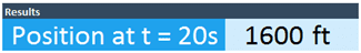
Now that the Position function is complete, you can use it in the spreadsheet to do calculations. First, use it to calculate the position at 20 seconds. Remember this function needs three arguments passed to it: x0, t1 and t2. Type in the function name, then use Ctrl-Shift-A to automatically populate the names of the arguments. The first argument, x0, is the initial position in cell C5; t1 is the lower bound in cell C6, and t2 is the upper bound in cell C7.
=Position(C5,C6,C7)
The Position function will give the result 1600 feet after 20 seconds.
Of course, the function can also be used to calculate the position at many different times. The worksheet already contains time and velocity data. For the position column, the arguments will be entered in a slightly different way. The initial position and the initial time are the same as above. You can begin the function:
=Position(C5,C6,
Both of these arguments need to be made absolute references using F4 because they’ll be the same for every time point in the table. However, the t2 argument will change as you go down the table, so you can simply click within cell B17 and leave that as a relative reference.
=Position($C$5,$C$6,B17)
Select this cell and double-click the fill handle to fill the formula down the column. This will give you the same end position of 1600 feet, but it also gives all the position and velocity data points in between. You can plot these together. Select all three columns and insert a scatter chart. The velocity data are much smaller numbers than the position, so plot those on a secondary axis. Right-click the velocity data and choose Format Data Series. Select Plot Series On Secondary Axis.
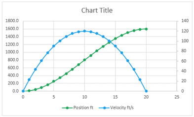
You can see that when the velocity is near zero, the slope of the position curve is flat. The position increases more rapidly as velocity increases, and eventually gains more slowly as the velocity begins to drop again. Finally, when the velocity is zero again, the position stops increasing.